Athans Blog

The crucial question in finance is why are asset prices different from each other? No-Arbitrage Pricing Theory indicates Stochastic discount factor (SDF) explains difference in asset prices. Yet the fundamental problem of asset pricing is what is the SDF?

The challenges of finding the SDF are:

1. Big Data: SDF should depend on all available economic information
2. Non-Parametric: Functional form of SDF is unknown and likely complex
3. Dynamics: SDF needs to capture time-variation in economic conditions
4. Weak Signal: Risk premium in stock returns has a low signal-to-noise ratio

Can Machine Learning help on this issue? Machine Learning methods are very flexible in dealing with big data, but asset prices in efficient markets are dominated by unforeseeable news. This paper however disciplines the machine learning algorithm with No-Arbitrage constraint and will strongly improves the signal.

Motivation

The conceptional challenges in asset pricing could be summarized into:

• What is the functional form of the SDF based on the information set?
  • Conventional example: Fama-French 5 factor model
  • Problem: Linear form could be miss-specified and there are 100 more potential characteristics out there
  • Solution: General non-parametric model with variable selection
• What are the test assets?
  • Conventional example: 25 Fama-French double-sorted portfolios
  • Problem: Selected SDF might only work on these test assets
  • Solution: All stocks and all possible characteristic based portfolios are taken into consideration to form the test assets
• What are the states of the economy?
  • Conventional example: NBER recession indicators
  • Problem: It includes 100 macro-economic time-series with complex dynamics
  • Solution: Extract a small number of state processes using complete dynamics of a large number of macro-economic time-series.

This paper estimates the SDF with deep neural networks, with the crucial innovation of including no-arbitrage condition in the neural network algorithms and combine three neural networks in a unique way. The key properties of this SDF estimator are:

1. Non-linearity: captured by the Feed-forward network
2. Time-variation: Recurrent network (LSTM) finds a small set of economic state processes.
3. Pricing all assets: Generative Adversarial Network (GAN) identifies the states and portfolios with the most unexplained pricing information
4. Signal-to-noise ratio: No-Arbitrage conditions applied to all three networks above to improve the risk premium signal.

This paper propose a model to find the optimal portfolio that empirically outperforms all benchmark models out of sample with an annual Sharpe Ratio of 2.6. The model explains 8% of variation in individual stocks and explains over 90% of average returns for characteristics managed portfolios.

The authors also cast some insights into the structure of the SDF:

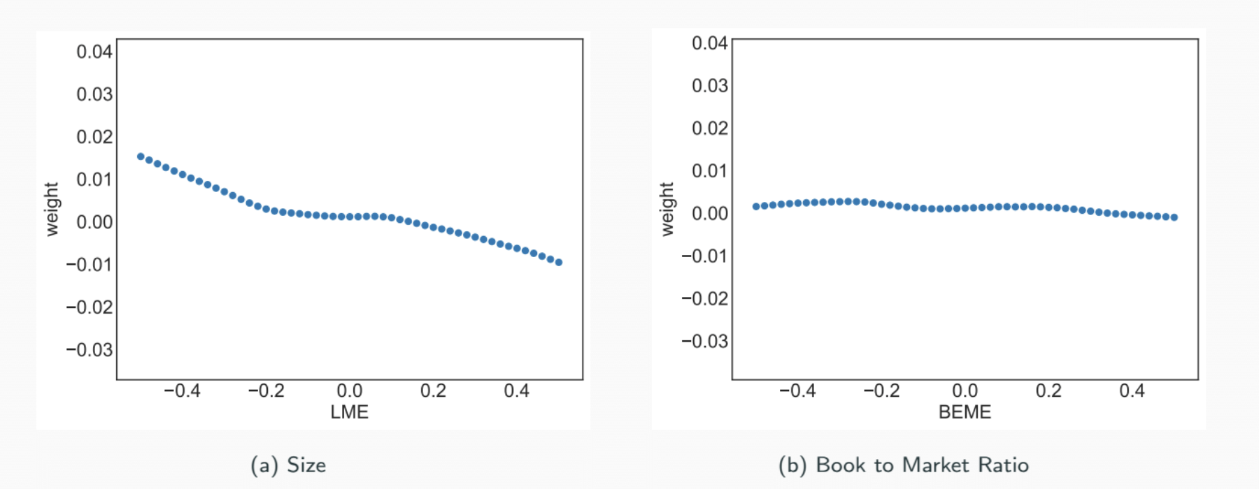
• Characteristics in isolation are approximately linear which explains why factor model makes sense
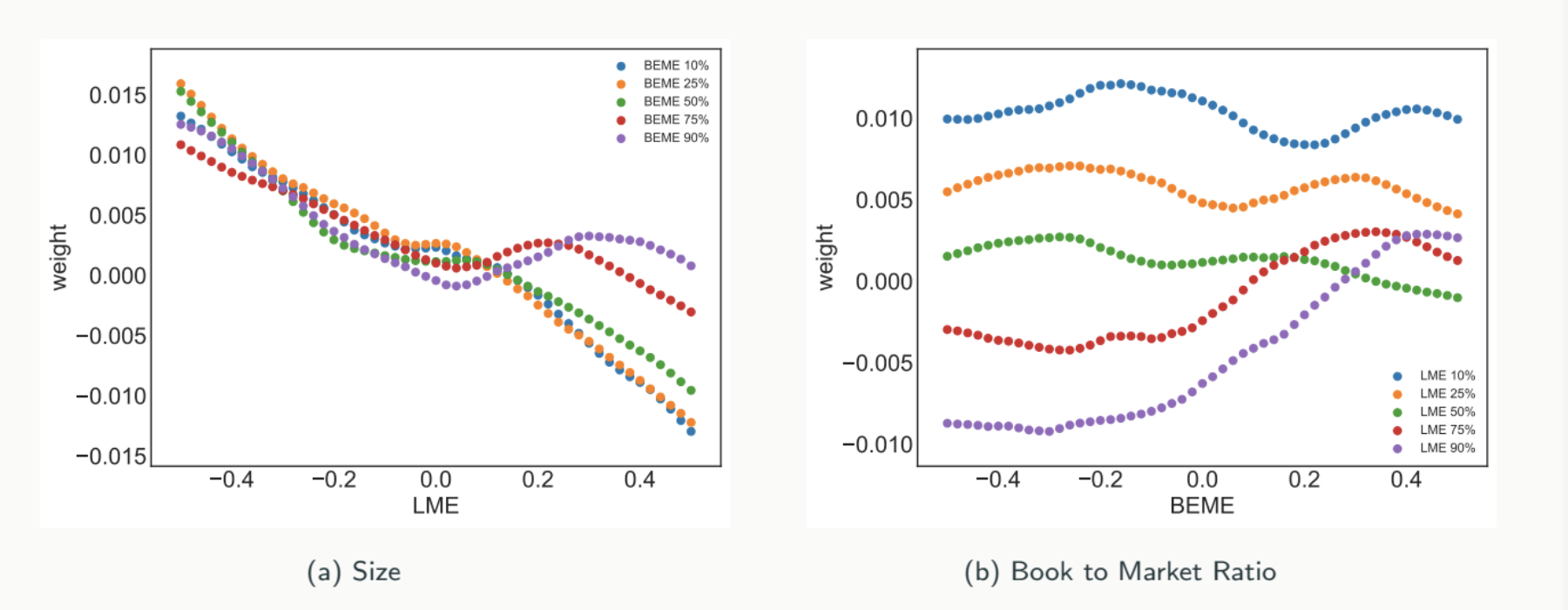
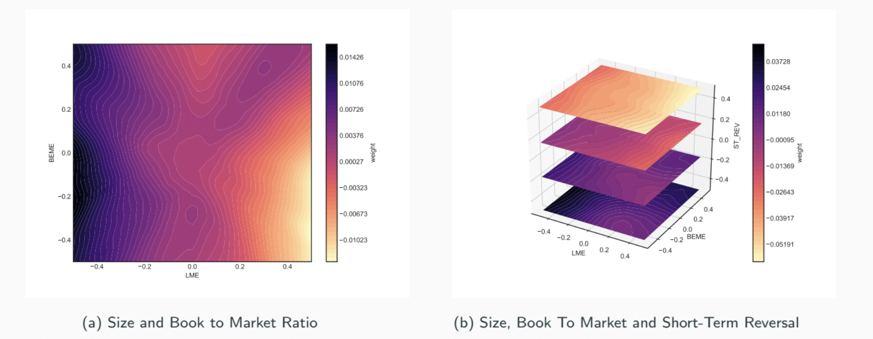
• However Non-linear interactions between firm information matter in finding SDF.
• Macro-economic states matter in finding SDF.
• SDF structure is stable over time based on 25 years of test data without refitting
• All classical firm characteristics relevant with price trends and trading frictions are the most important.

In addition, Off-the-shelf machine learning methods often perform worse because economic constraints matter. Machine learning combined with economic model structure works significantly better, such applications could be found in the below categories:

• Deep Learning for predicting asset prices: Predicting future asset returns with feed forward network
• Deep Learning auto encoder: Constructing low dimensional non-linear factor structure
• Linear or kernel methods for asset pricing of large data sets: Methods including Instrumented PCA, Risk premium PCA, mean-variance with regularization, and group lasso.
• Tree based learning for general non-linear interactions: Asset-Pricing Trees.

Model

According to the fundamental no-arbitrage condition we have $E_t[M_{t+1}R_{i, t+1}^e]=0$ For all $t=1,...,T$ and $i=1,...,N$ where $R_{i, t+1}^e=R_{i, t+1}-R_f$ equals the excess return at time t+1 for asset $i=1,...,N$; $E_t[.]$ is the expected value conditioned on information set at time t; $M_{t+1}$ is the stochastic discount factor (SDF) at time t+1.If we had some $F_t$-measurable variable $I_t$ , we could imply the unconditional moments from conditional moments $E[M_{t+1}R_{i, t+1}^eI_t]=0$

Without loss of generality SDF is projection on the return space as $M_{t+1}=1-∑_{i=1}^N w_{i,t}R_{i, t+1}^e$, where SDF portfolio $F_{t+1}=∑_{i=1}^N w_{i,t}R_{i, t+1}^e$ has the highest conditional Sharpe Ratio; portfolio weights $w_{i,t}$ are a general function of macro-economic information $I_t$ and firm-specific characteristics $I_{i,t}$ : $w_{i,t}=w(I_t,I_{i,t})$. This function would need non-linear estimator with many explanatory variables.

No-arbitrage condition is equivalent to factor representation of $R_{t+1}^e=\beta_tF_{t+1}+e_{t+1}$.

Our objects of interest include the following:

• The SDF portfolio $F_t$ And its portfolio weights $w_{i,t}$
• The risk loadings $\beta_{i,t} = cov_t(R_{i, t+1}^e, F_{t+1})/var_t(F_{t+1})$
• The unexplained residual $\hat{e_t}=(l_N-\beta_{t-1}(\beta_{t-1}^T\beta_{t-1})^{-1}\beta_{t-1}^T)R_T^e$

Estimation

We need to estimate SDF weights function w to minimize no-arbitrage moment conditions $E[M_{t+1}R_{i, t+1}^e\hat{I_t}]$ for a set of conditioning variables $\hat{I_{i,t}}=\hat{g}(I_t,I_{i,t})$. We construct the empirical no-arbitrage loss function given $\hat{I_{i,t}}$ to be

$$L(w|\hat{g},I_t,I_{i,t})=1/N*∑_{i=1}^NT_i/T⎜1/T_i∑_tM_{t+1}R_{i, t+1}^e\hat{g}(I_t,I_{i,t})⎟^2$$

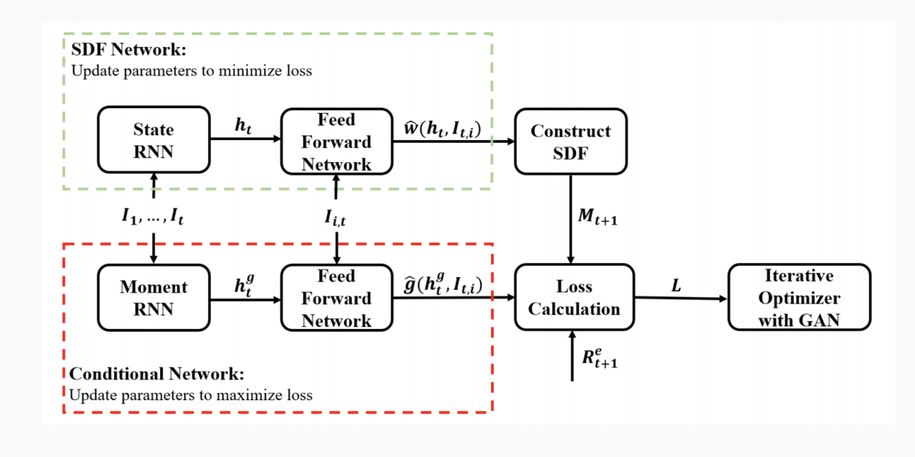
We use a feed forward network to estimate $w_{i,t}$ for given $\\hat{I\_{i,t}}$ (or $\hat{g}(I_t,I_{i,t})$ ), the finance intuition behind it is that $R_{t+1}^e\hat{I_{i,t}}$ form the characteristic managed portfolios, for example $g$ might build size/value portfolios as test assets, thus the problem of finding optimal “instruments” equals the choice of test assets. Now the problem is that model implies infinite number of moment conditions of $\hat{I_{i,t}}$. Imposing all functions forms would be infeasible, how do we choose the conditioning variables $\hat{I_{i,t}}$ as general functions $\hat g$ of the macroeconomic and firm-specific information then? We train a Generative Adversarial Network (GAN) to choose it.

We design two networks to play a zero-sum game:

1. SDF network ($\hat w$) constructs the SDF $M_{t+1}$
2. Conditional network ($\hat g$) generates conditioning variables $\hat{I_{i,t}}$

We alternatively update the two networks: 1) For a given set of conditioning variable $\hat{I_{i,t}}$ , SDF network is updated to minimize the loss (least pricing error). 2) For a given estimation of the SDF, Conditional network finds $\hat{I_{i,t}}$ With the largest loss (most pricing error).

In short, for a candidate SDF $M$ the adversary $g$ constructs the test assets (and states) where $M$ has difficulty pricing:

$$min_Mmax_g∑_i||∑_tM(I_t,I_{i,t})R_{i, t+1}^eg(I_t,I_{i,t})||^2$$

The intuition is to find the economic states and test assets with the most pricing information, for example if SDF is the $M$ is Fata-French 5 factor SDF, then g constructs momentum portfolios.

From the econometrics perspective, conventional General Method of Moments (GMM) extracts optimal instruments based on efficiency, but it is not feasible for large number of potential parameters and it assumes test assets would identify SDF parameters. Our GAN approach looks for optimal instruments based on robustness, it is now feasible for large set of instruments and parameters, and it finds test assets and identify SDF parameters simultaneously.

Now the next big question is finding hidden macroeconomic states. Examples of macroeconomic time series with standard transformation indicate macroeconomic states are time-series dependent. The problems with economic time-series data are:

• Time-series data is often non-stationary ⇒ transformation necessary (first order differentiating)
• Asset prices depend on economic states ⇒ simple differencing of non-stationary data is not sufficient
• Macroeconomic data is strongly. time-series dependent ⇒ it has low dimensional structure

Our solution is to use Recurrent Neural Network (RNN) with Long-Short-Term Memory (LSTM) cells. LSTM could transform all macroeconomic time-series into a low dimensional vector of stationary state variables. The intuition is that RNN resembles a non-linear hidden state space model combined with non-linear factor model.

The whole model architecture looks like:

Empirical Results

We used 50 years of monthly observations from 01/1967 to 12/2016. The data include monthly stock returns for all US securities from CRSP and we only use stocks with all firm characteristics (around 10000 stocks). We use 46 firm-specific characteristics for each stock every month to formulate $I_{i,t}$ , then normalized to cross-sectional quantiles. We use 178 macroeconomic variables (124 from FRED, 46 cross-sectional median time-series for characteristics, 8 from Goyal-Welch) to formulate $I_t$. The training period is 20 years, validation period is 5 years, and testing period is 25 years.

We built two benchmark models to compare with:

1. Linear model: SDF portfolio weights $w_t=I_t\theta$ linear in characteristics. The intuition is that it is equivalent to perform mean-variance optimization on characteristic managed long-short factor portfolio $\hat R_{t+1}=I_t^TR_{t+1}^e$. To solve $\theta$ we want to consider whether to add regularization or not:

   1. OLS: Linear regression $\hat \theta = (\hat R^T\hat R)^{-1}\hat R^T1$
   2. EN: Elastic Net regularization (Kozak, Nagel and Santosh (2019)):

$$min_\theta||1/T\hat R^T1-1/T\hat R^T\hat R\theta||^2+\lambda_1||\theta||+\lambda_2||\theta||^2$$

2. FFN: Deep Learning return forecasting (Gu, Kelly and Xiu (2019)): we use only simple feedforward network to predict conditional expected returns $E_t[R_{i, t+1}]=\beta_{t,i}E_t[F_{t+1}]$. The conditional mean is proportional to SDF loading $\beta_{t,i}$. The empirical loss function we used to train the network is: $1/(NT)∑_{i=1}^N∑_{t=1}^T(R_{i,t+1}-\mu(I_t, I_{i,t}))^2$.

Combined with our previous model settings, our objects of interest are:

• The SDF portfolio $F_t$
• The risk loadings $\beta_t$
• The unexplained residual $\hat{e_t}=(l_N-\beta_{t-1}(\beta_{t-1}^T\beta_{t-1})^{-1}\beta_{t-1}^T)R_T^e$

Universally the Asset Pricing model performance is measured by:

• Sharpe ratio of SDF portfolio: $SR=\hat E[F_t]/ \sqrt{\hat {Var}(F_t)}$
• Explained variation:

$$EV = 1- (1/T∑_{t=1}^T1/N_t∑_{i=1}^{N_t}(\hat e_{i, t+1})^2)/(1/T∑_{t=1}^T1/N_t∑_{i=1}^{N_t}(R_{i, t+1}^e)^2)$$

• Cross-sectional mean R Square:

$$XS\_R^2=1-(1/N∑_{i=1}^NT_i/T(1/T_i∑_t\hat e_{i, t+1})^2)/(1/N∑_{i=1}^NT_i/T(1/T_i∑_t\hat R_{i, t+1})^2)$$

The below table lay out the results of our model GAN, forecasting FFN, linear EN and LS:

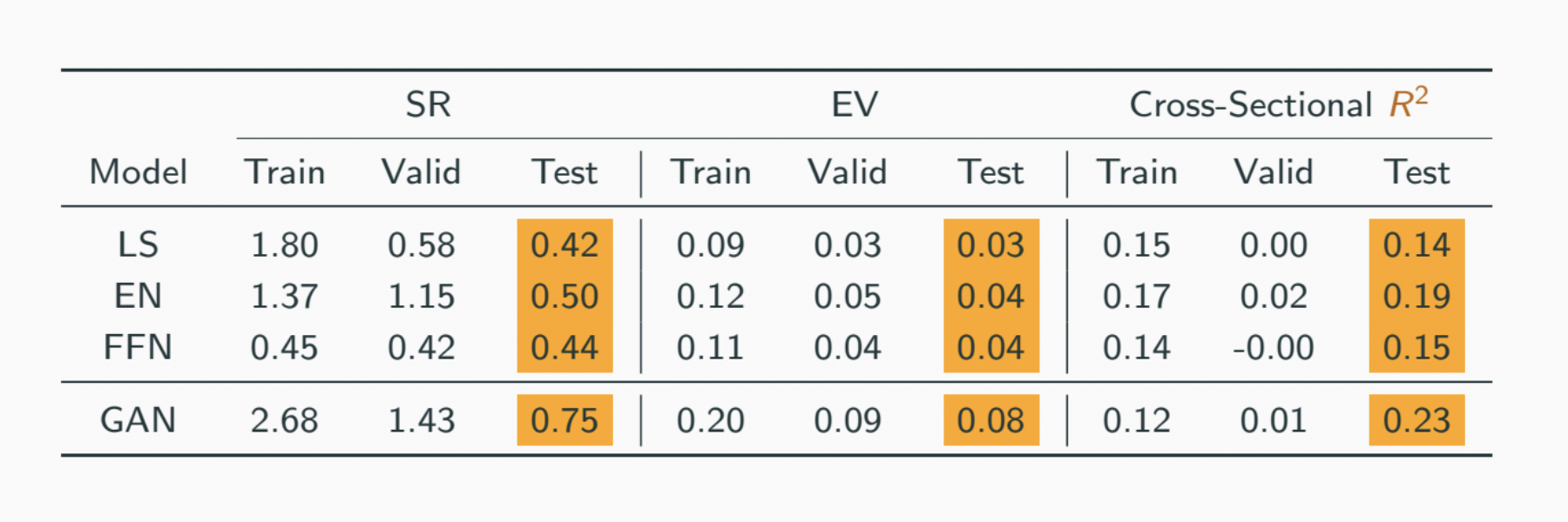
The annual out-of-sample Sharpe Ratio SR for GAN is 2.6, GAN explains twice as much (8%) of the variation in individual stocks than other models, GAN has explained higher fraction of cross-sectional average return too. Linear model (EN) outperforms forecasting FFN which indicates no-arbitrage condition matters!

We also compare performance of models with different macroeconomic variables, Sharpe Ratio of SDF for different inclusions of macroeconomic information are as below:

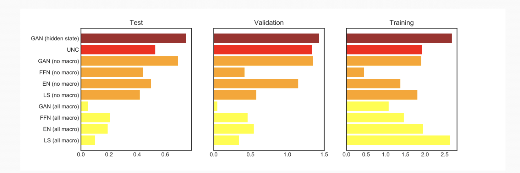
As we show, GAN (hidden states) is our reference model which has the highest Sharpe Ratio. “no macro” uses only firm characteristics, “all macro” uses standard transformation of macroeconomic time-series without LSTM. Needless to say that macroeconomic hidden states matter here.

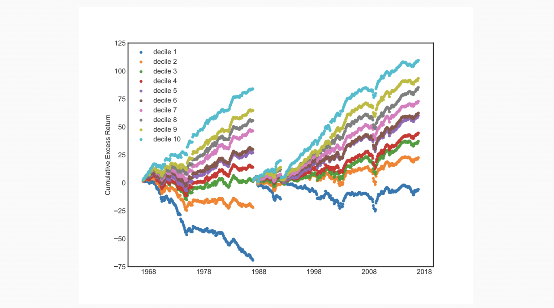
With the plot of cumulative excess returns of $\beta$ Sorted decile portfolios for GAN shows that risk loadings predict future stock returns.

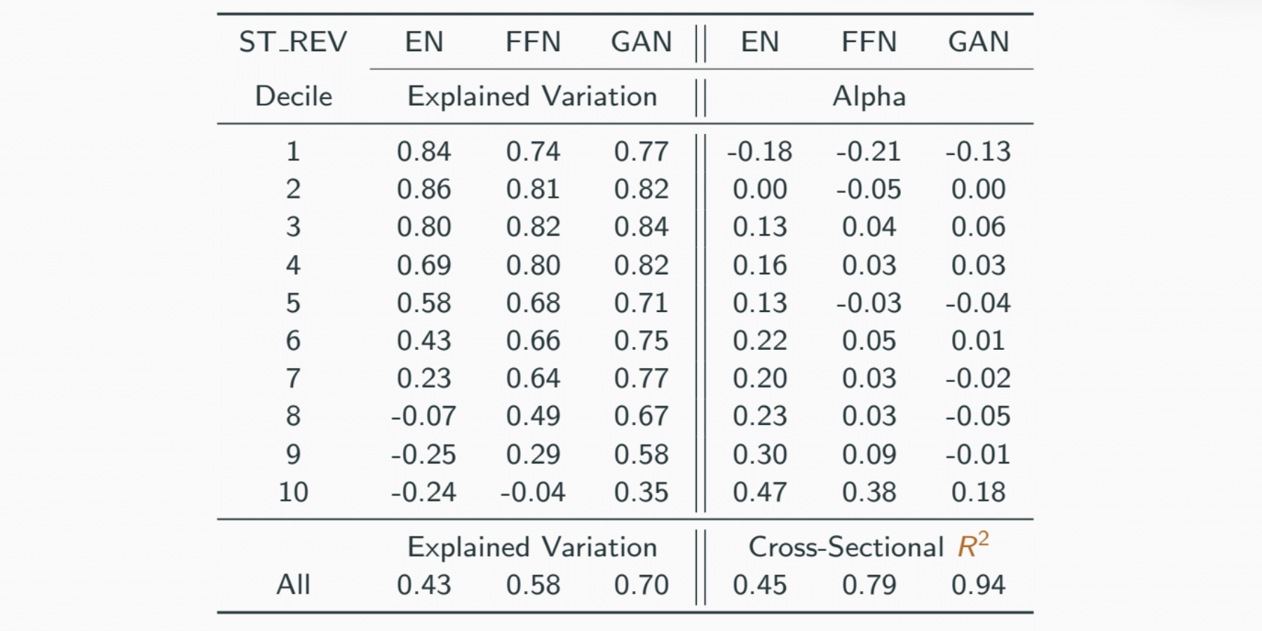
The table below showed explained variation and pricing errors from different models for short-term reversal sorted portfolios (out-of-sample results for value weighted decile portfolios). GAN explains extreme quantiles better.

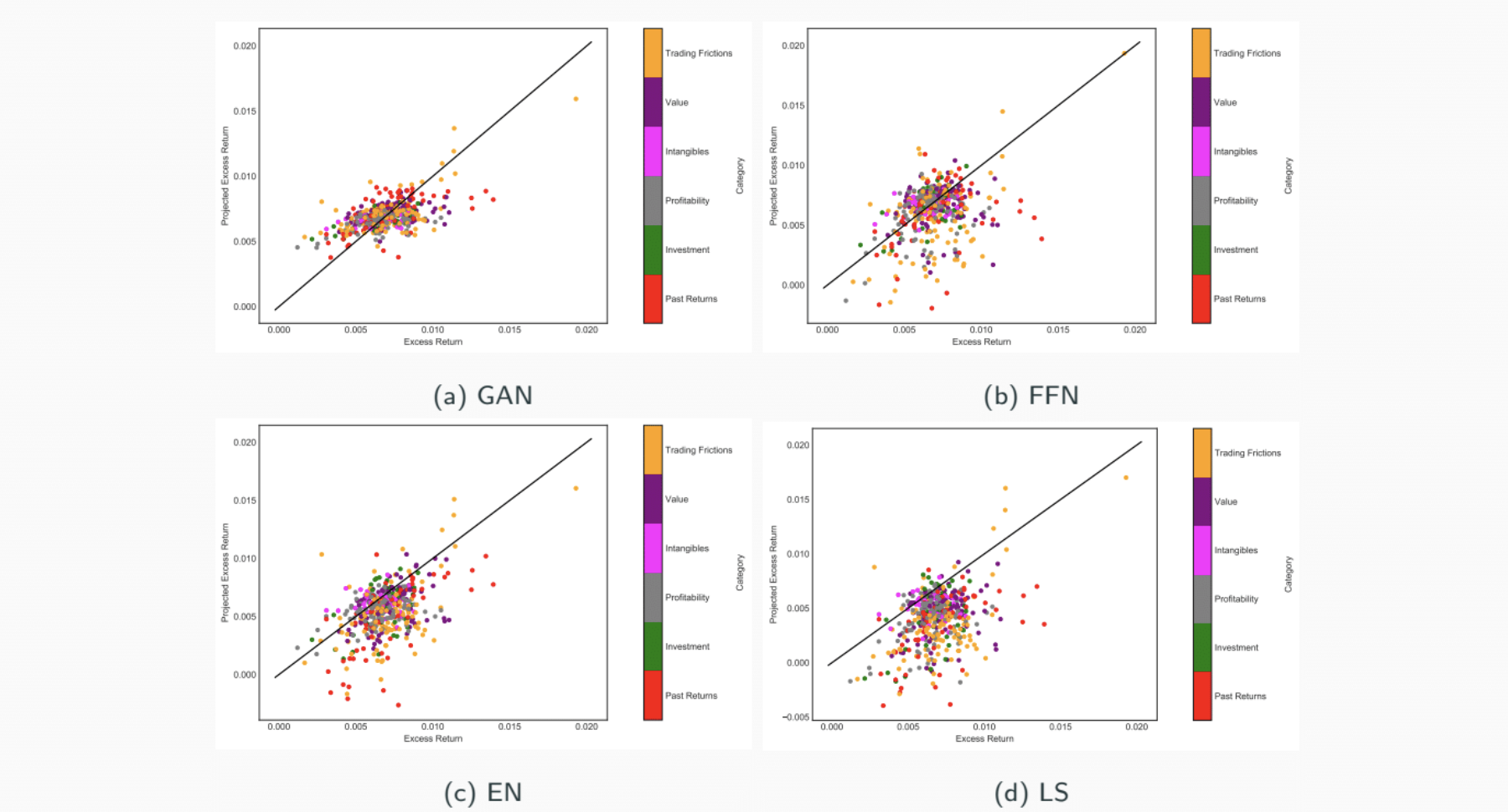
In addition, if we examine the predicted and average returns for value weighted characteristics sorted portfolios (out-of-sample result for 46 characteristics sorted decile portfolios). GAN always has cross-sectional $R^2 > 90\%$ for each 46 decile portfolios which means GAN explains the cross-section of average returns better.

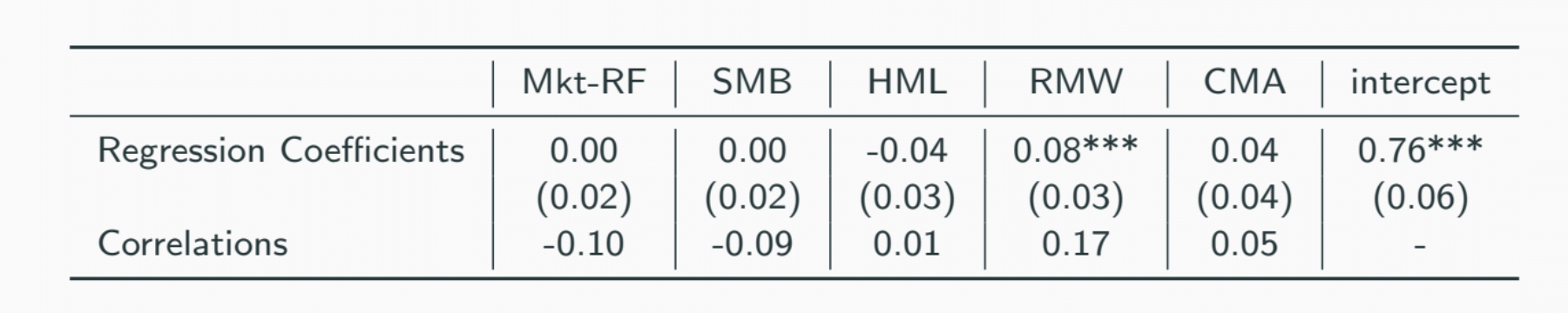
If we look at the out-of-sample correlation and regression of GAN SDF on Fata-French 5 factors models, it states that Fata-French factors do not span GAN SDF.

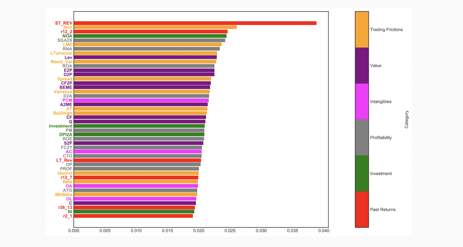
Now taking a perspective of characteristics importance, from the plot with GAN characteristics importance ranking in terms of average absolute gradient, we know that price trends and trading frictions are most relevant and all categories represented among top 20 variables.

Lastly we show SDF weight with regards to different functions of size and book-to-market ratio. If we pick SDF weight $w$ as 1-dimensional function keeping other covariates at their mean values, the chart implies size and book-to-market have close to learn effect on SDF weight.

If we pick SDF weight $w$ as 2-dimensional function keeping other covariates at their mean values, the chart implies complex interaction between multiple variables.

If we pick SDF weight $w$ as 2-dimensional function keeping other covariates at their mean values, the chart still implies complex interaction between multiple variables.

Conclusion

We come up with a novel combination of deep neural networks to estimate the pricing kernel, the key innovation is to use no-arbitrage condition as criterion function. The time-variation is explained by macroeconomic states and firm characteristics. The test assets with most pricing information are selected by adversarial approach (GAN). This is a general asset pricing model that includes all other models as special cases.

From empirical results, our GAN model outperforms benchmark models. The model have incorporated non-linearities matter for the interaction, but those characteristics in isolation is approximately linear. Macroeconomic states matters and adding them improve the model out-of-sample performance. SDF predicts future returns and explains cross-sectional average returns, its structure is stable over time, SDF portfolio itself is highly profitable. Finally, GAN framework is complementary to conditional multi-factor models.