
This paper combines machine learning with investment objectives. It extracts complex signal from vast many variables and could easily include relevant constraints, e.g. removing illiquid assets or penny stocks. The model which the author comes up with is easily interpretable and simple to use, and the economic structure the author lays helps with the low signal to noise ratio in stock returns.
Introduction
Academics and practitioners have two perspectives on investments, but they actually share the same fundamental problem with the same solution. It is better to build some translations channels between the two parties first:
- Stochastic Discount Factor (SDF) = optimal portfolio with highest Sharpe ratio
- Basis/test assets = simple (long-only) investment strategies for optimal portfolio
- Sorting portfolios = (non-linear) prediction of future returns
Academically this paper generalizes sorting to find basis/test assets to construct the Stochastic Discount Factor. From the practitioner’s angle, this paper develops a new way of predicting stock returns and constructing simple investment strategies, and then shows how to combine them to a portfolio with highest Sharpe ratio.
Broadly speaking, academic finance research concerns about the efficacy of asset pricing, professors want to:
- Test assets for the accuracy of the asset pricing models
- Construct better asset pricing models
- Understand the source and size of risk premium
Practitioners are more intrigued by the inefficacy of asset pricing, hedge fund managers in actual investment:
- Find profitable portfolios not explained by common risk factors in such model
- Identify mispricing = alpha opportunities in markets
Ever since the publishing of the Fama French 3 factor paper, sorting becomes the conventional approach to construct test assets where people use to test the efficacy of new signals. If we hold the prior that one characteristic of the assets (let’s say Book-to-Market) is informative about expected returns, the sorting portfolios provides a nonparametric estimator of conditional mean returns, which is equivalent to kernel regression to predict returns. Sorting delivers simple investment strategies, and it is the foundation to construct risk factors (high bucket minus low bucket represents the value factor).
If we extend our prior to multiple characteristics, the state of the literature is to do so called “double sorting” where sorting portfolio is routinely used to create cross-sections buckets based on these 2 characteristics. If our prior consists of more than 3 characteristics, then we stack several cross-sections buckets together, for example 25 size and value + 10 momentum + 10 accruals.
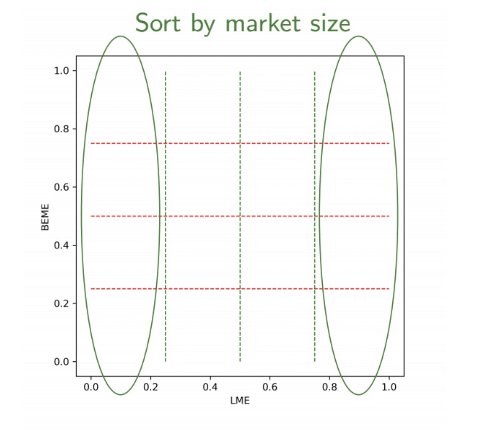
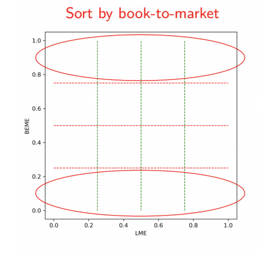
In sum sorting yields the test assets we used to form the portfolio to test the efficacy of the firm characteristics. Now the apparent challenges for the sorting approach are:
- Single sorting ignores any interactions between characteristics
- Multiple sorting is limited to coarse double or triple interactions
- Not considering firm distribution, some buckets will form empty and unbalanced portfolios
We also argue that the success of simple long-short factors is due to the overly simplistic test assets from the sorting approach, because the sorting portfolio diversify the idiosyncratic noise and are easy to interpret.
We propose the Asset Pricing Trees (AP-Trees) which is cross-section of basis assets that reflect all the information including interactions and non-linearities, relying on the two steps:
- Tree-sorted portfolios: creating managed portfolios with arbitrary interactions
- Pruning the trees: selecting portfolios that are the most relevant for asset pricing
The advantages of AP-Trees are that it’s simple and interpretable, it’s a generalization of prevailing sorting methodology. It takes into account the arbitrary interactions among characteristic s and non-linearities, while pruning alleviates the curse of dimensionality. It provides new basis assets to test asset pricing models and offers investment opportunities not spanned by common risk factors.
For the empirical results of the AP-Trees, it has higher Sharpe Ratios than sorting portfolios or conventional factors, and is harder to price cross-sectionally, because standard sorting and stacking doesn't reflect well the underlying information and presents too low a bar. In short better results are achieved by including economic structure in machine learning algorithm.
Sorting, Trees, and Forest
A tree of depth can be formed based on characteristics and the rule of 50/50 splits:
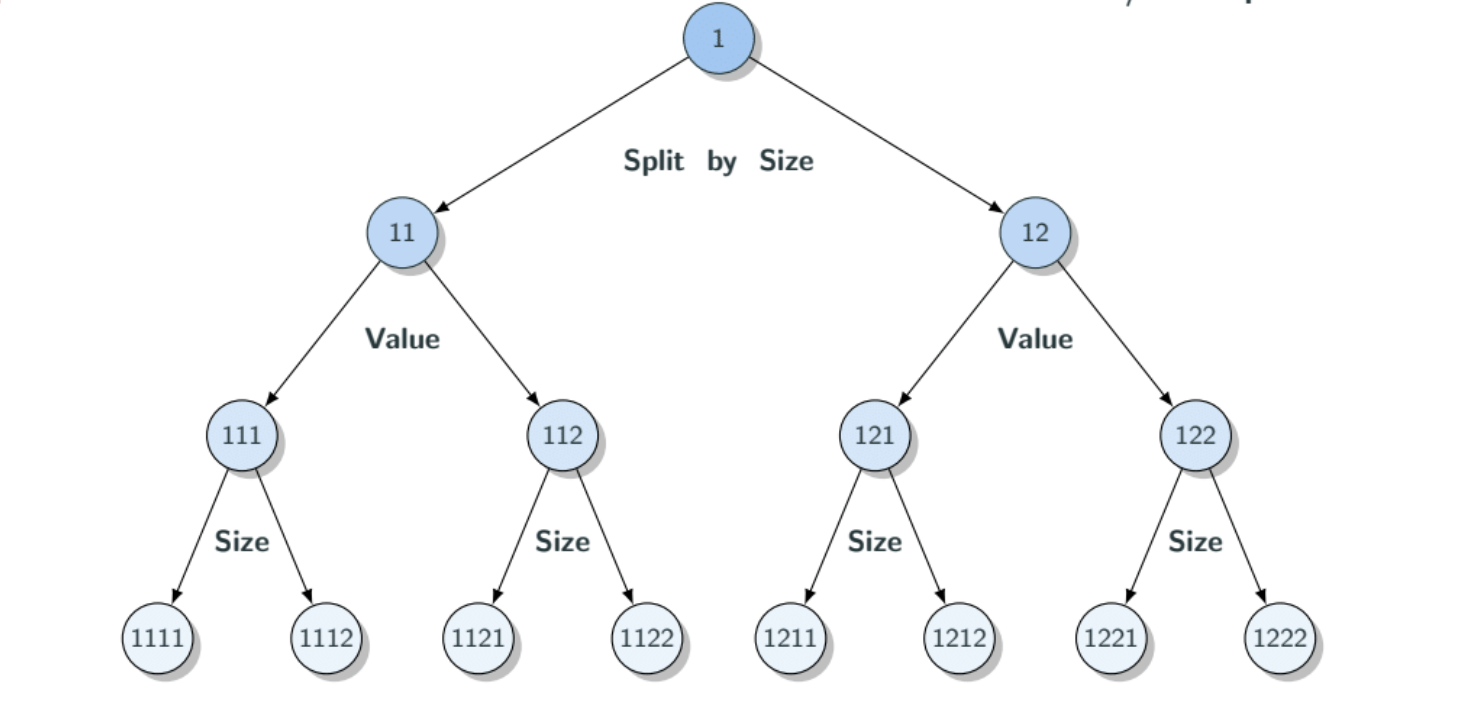
The simplest trees rely on the 50/50 split within each group of the assets. Conditional on the order of splits, we could generate Subtrees, with each subtree yielding non-intersecting portfolios. The Asset Pricing Trees (AP-Trees) contain portfolios altogether, with Stocks in each leaf node independent of k.
The Tree-based portfolios are the result of conditional splits, thus they reflect join distribution of characteristics without the need for parametric modeling. This is important because many characteristics have a complicated joint distribution, meaning that focusing on unconditional quantiles can produce either empty or too dense portfolios.
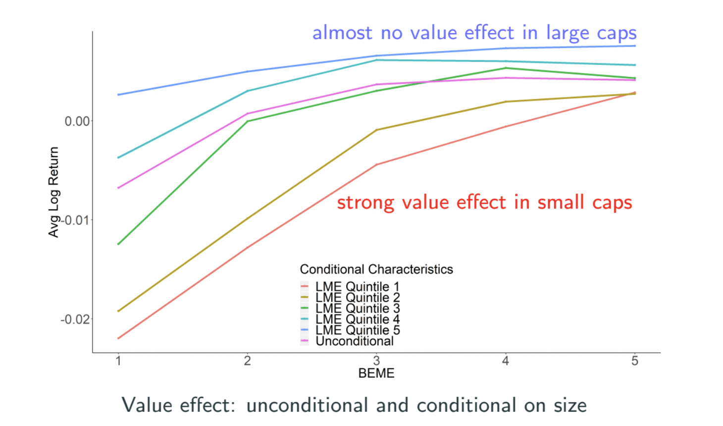
We have the dimensionality curse in AP-Trees, with only 2 characteristics and depth of 3 we have Subtrees, within each having portfolios. This is a total of 64 (intersecting) portfolios. With 3 characteristics and depth of 4 we will have 1296 final portfolios. Apparently we need some sort of dimension reduction (portfolio selections) on these 1296 final leaf nodes.
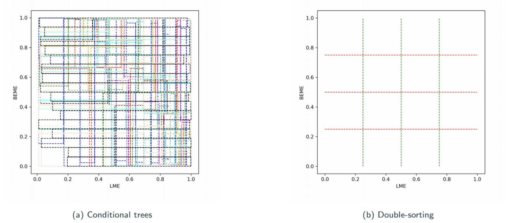
The tricky part is that usual techniques for portfolio selections (pruning) are not applicable here, since stocks with the same expected return could have very different features, for instance small stocks within value firms and large cap stocks within growth firms.
Let’s return to the tree example shown before. According to the standard bottom-up pruning approach, we want to compare the returns of 1111 and 1112, if they are different we keep them separate.
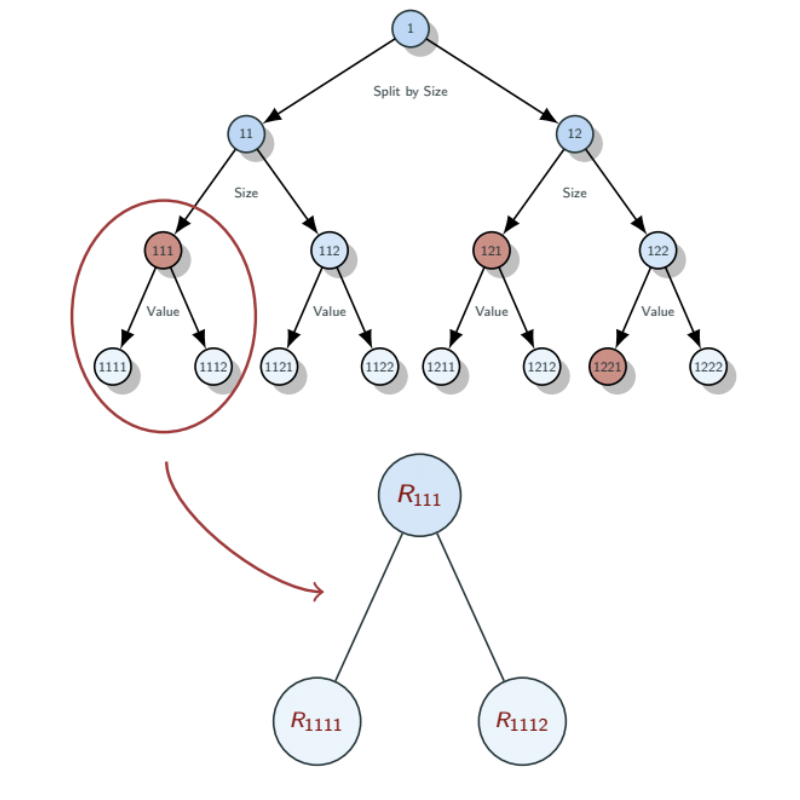
Now the problem is when selecting blocks for the SDF, our goal is to find the best set of basis assets (leaf nodes) with which together they should give the highest Sharpe Ratio. Whether the set is optimal depends on other nodes because the portfolio is nothing but assigning weights to stocks. That means pruning cannot be local, we need another way to take into account other nodes.
Conventional machine learning tree pruning (bottom-up approach) is local in nature and works only if the current split doesn't affect other nodes. Our object is to find the optimal basis assets from the tangency portfolio, and this is a global decision problem where comparing tree portfolios locally is not sufficient. Pruning reflects the risk of not only the mean return () but also the covariance (). Our approach is the Asset Pricing Pruning which is to create optimal mean-variance portfolios with shrinkage and applied to all the final and intermediate nodes of the tree portfolios.
To elaborate this solution, we take all the final and intermediate nodes from all the trees to construct the tangency portfolio on a robust and sparse mean-variance efficient frontier:
- Construct a portfolio frontier on training data with elastic net (under uncertainty)
Tuning the hyper parameters via the validation data: target return $\mu_0$, sparsity lasso shrinkage $\lambda_1$, ridge shrinkage $\lambda_2$.
- Choose the robust tangency portfolio by selecting tuned parameters on the validation data set.
The key elements in this solution are:
- Lasso: selecting a small number of basis assets (sparsity)
- Ridge: stability in covariance estimation
- Target Return: combining tangency portfolio with the minimum-variance portfolio, and also shrinking expected returns toward their cross-sectional average
This is to say that we come up with a fast and efficient algorithm that converts portfolio optimization to a regularized regression setup.
Let’s throw some intuition for these shrinkage components (and exclude lasso for now). We first know that Unconstrained SDF – the tangency portfolio of conventional mean-variance optimization – breaks down in large dimensions.
Meanwhile our approach could be compared to a robust tangency portfolio and 2-fund separation theorem.
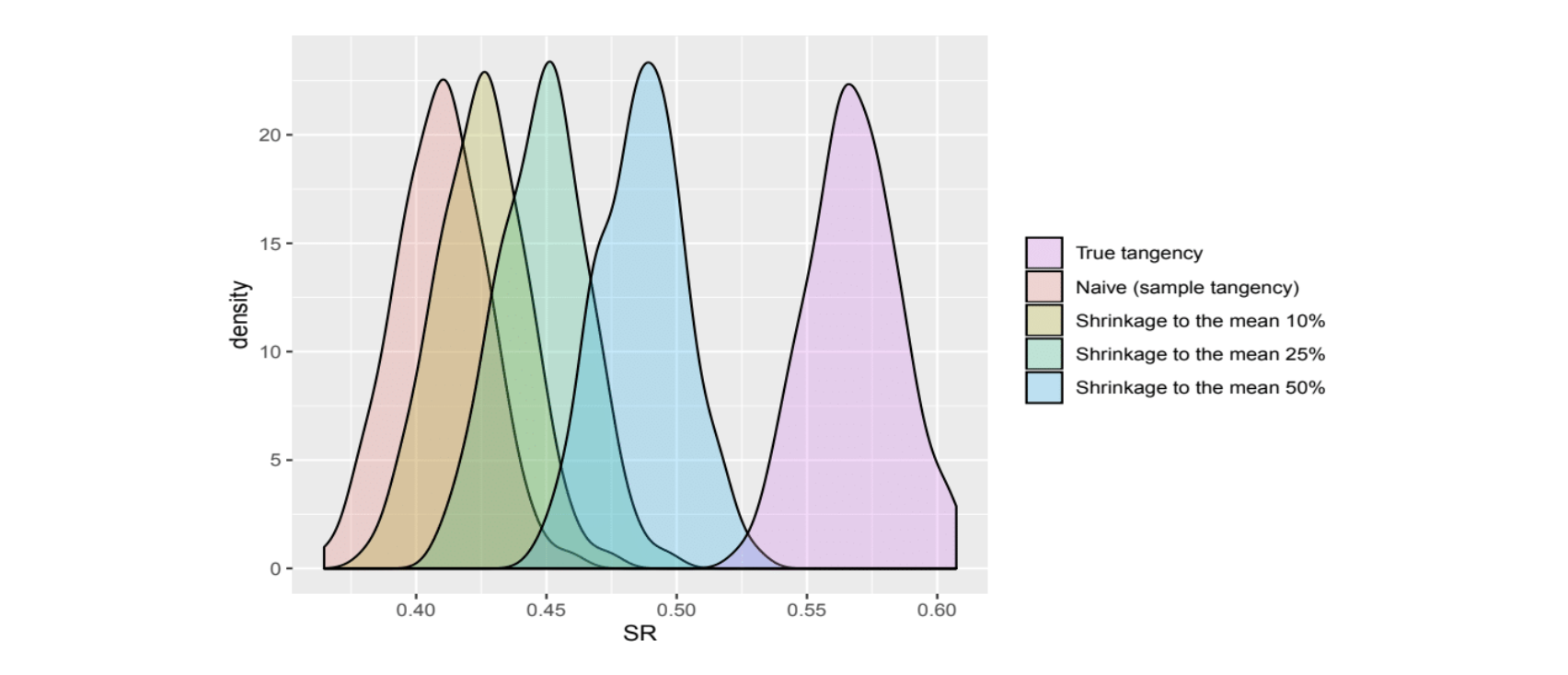
We apply shrinkage in the covariance matrix and sample mean towards the average. Covariance matrix shrinkage is nothing new and we could consider mean shrinkage as combining tangency portfolio with the minimum-variance portfolio. There is a one-to-one mapping between the target mean and mean shrinkage , the extreme sample means are likely wrong so we pulled them toward the cross sectional average. Thus we are actually sacrifice some returns in exchange for much smaller variance (a typical bias variance tradeoff), analogue to Bloomberg’s adjusted beta shrunk towards 1. If we generate iid stocks with same know variance but different (estimated) mean returns, through simulation of out-of-sample Sharpe ratio for tangency portfolios, we see a clear edge with shrinkage.
Another theoretical justification for the Asset Pricing Pruning comes from the robust estimation interpretation. If we are not confident about the empirical estimates of covariances and expected returns, Robust mean-variance optimization is equivalent to finding the mean-variance efficient solution under a worst case outcome for estimation uncertainty. Uncertainty sets for estimated Sharpe ratio, mean and variance are bounded:
- Uncertainty in Sharpe ratio is controlled by mean shrinkage
- Uncertainty in mean ratio is controlled by lasso shrinkage
- Uncertainty in variance is controlled by ridge shrinkage
In this sense, we build optimal portfolios for cautious investors who dislike uncertainty.
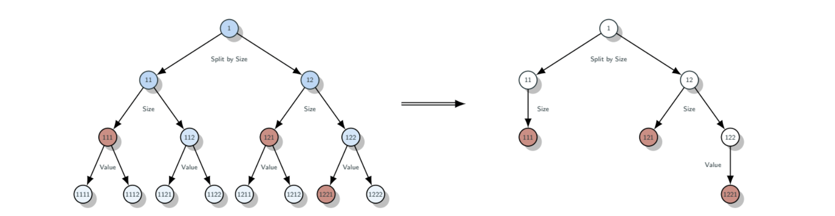
So what did we achieve after pruning? We group stocks together with the same SDF exposure to form a smaller tree, and the magnitude of pruning is adjusted for portfolio depth.
Cross-Sections Empirics
The authors use the monthly stock returns from CRSP merged with Compustat from January 1964 to December 2016 (53 years) as the data sample. We also gathered 46 firm specific characteristics and consider a short list of 10 characteristics out of those: Size, Value, Operating Profitability, Investment, Momentum, Short-term Reversal, Long-term Reversal, Accrual, Asset Turnover, and Idiosyncratic Volatility. Through these 10 characteristics the authors form the basic set by picking Size plus two others, thus there will be 36 cross-sections results. The same portfolio approach will be applied to all the basis assets such that all the difference in results will be coming from using trees or triple sorting.

The whole data is split to training, validation, and testing set, in which:
- Training: data is used to estimate the 40 basis assets metrics in the AP-Tree, then construct the weights of SDF based on the AP-Tree. The triple sorting test portfolios are formed by triple sorted with 32 assets (only one size split) and with 64 assets (two size splits).
- Validation: data is used to select tuning parameters
- Testing: data is used to conduct out-of-sample tests for AP-Trees and overall portfolios (SDF) on their Sharpe ratios, alphas and their t-stats, etc. The alphas (pricing errors) was calculated based on the following:
- 11 Factors which consist of the market factor plus all 10 cross-sectional specific factors
- 4 Factors which consist of market factor plus the 3 picked cross-sectional specific factors
- Fama-French 3 and 5 factors.
Note that all the basis assets are value-weighted portfolios and exclude extreme single-sorted basis assets. The AP-Trees have a fixed depth of 4 with the pre-chosen 3 characteristics.
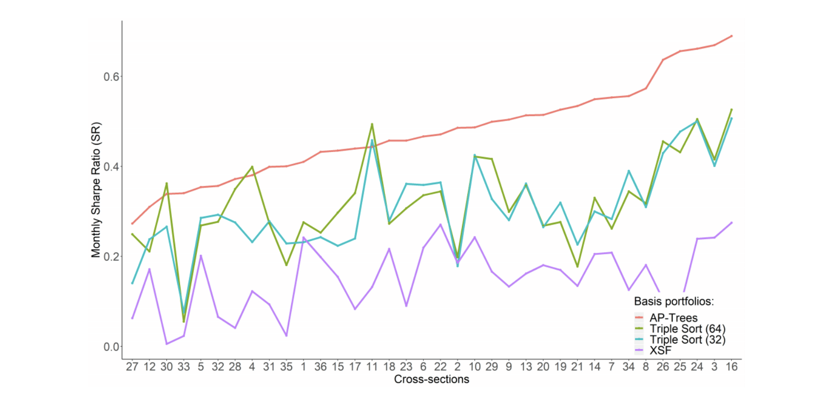
The empirical results shows that mostly out-of-sample Sharpe Ratios of mean-variance efficient portfolios for AP-Trees win over the basis portfolios formed from triple sorting and XSF (cross sections sorted by the SR of AP-Trees)
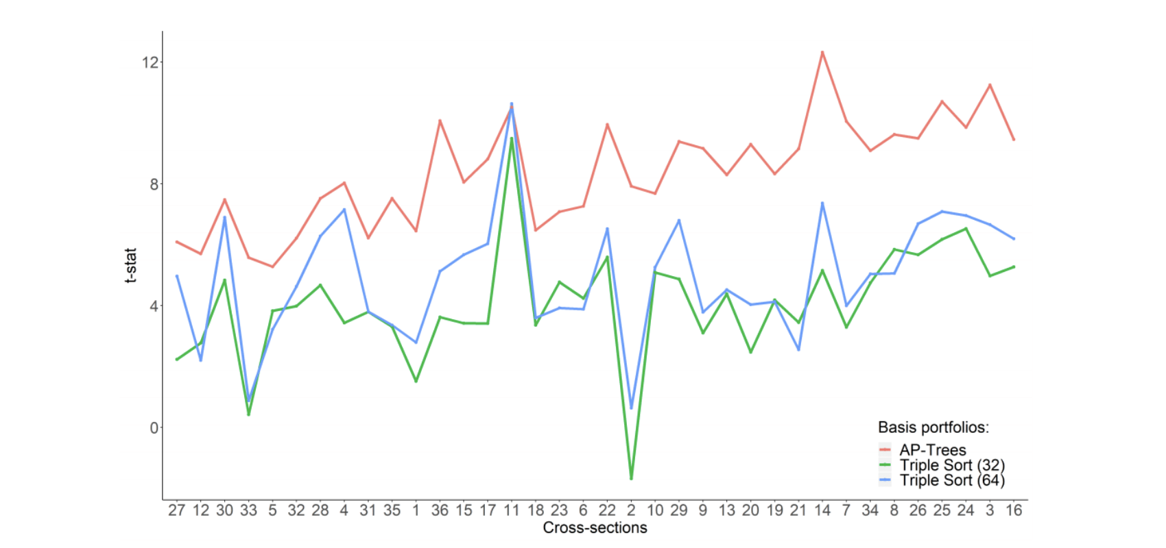
The t-stat of the Tree-based SDF alpha relative to market and 3 cross-section-specific factors is high, meaning AP-Tree based SDF is unspanned by traditional long-short factors.
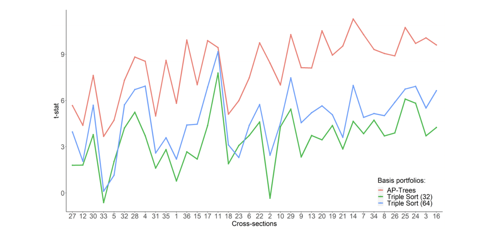
Similar results are shown when we calculate alpha relative to the 11 Factors model.
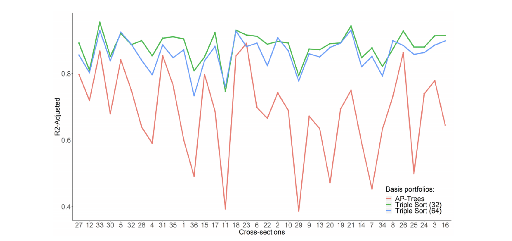
Furthermore from the R squared between cross-sectional pricing of portfolios and cross-section specific factors, we show that common risk factors cannot price AP-Trees based SDF within cross-sections (low R squared), while Triple Sorting portfolios are easier to price than AP-Trees based portfolios for all the characteristics.
Zooming into the results
We have shown the empirical results of the 36 cross-sections testings, now let’s delve into one specific example which picks size, operating profitability and investment as the characteristics being tested. We have constructed AP-Tree with 40 portfolios (as before) and with 10 portfolios (with finer pruning), it is shown that 10 AP-Tree portfolios capture the same pricing information as 40, but the alpha t-stat is twice as large for both AP-Trees than sorting based portfolios.
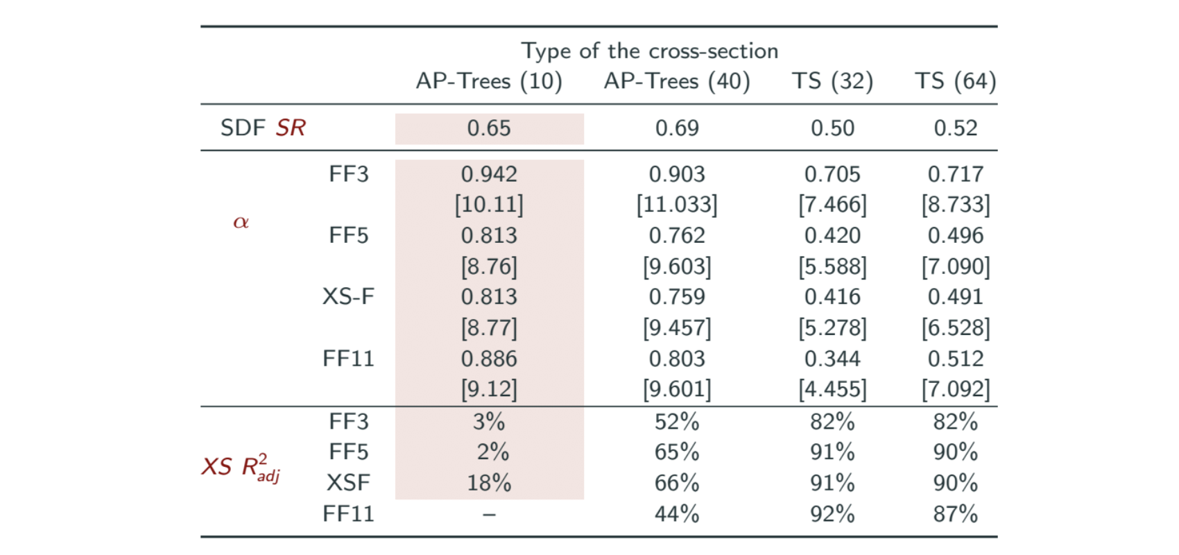
So how many basis assets do we need? From the charts below we know that 10 AP-Tree portfolios has the same Sharpe Ratio as 40, whether ex ante or ex post.
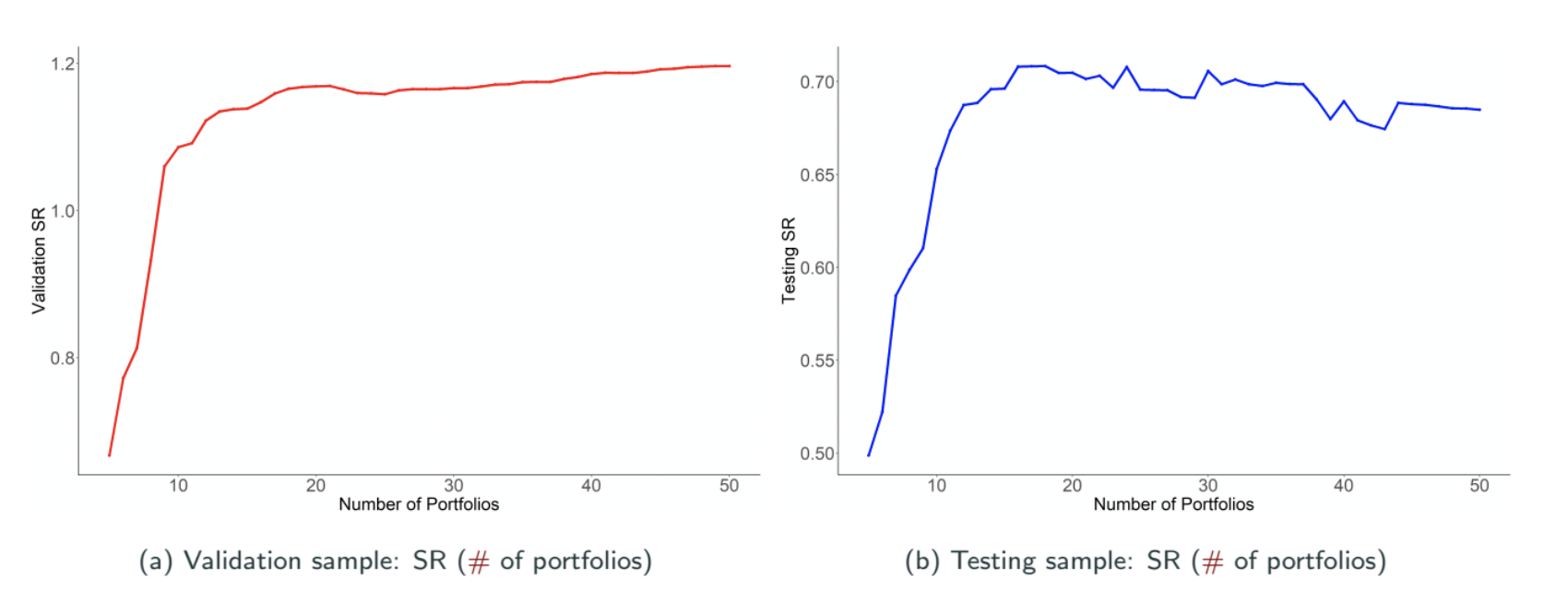
The variance shrinkage and mean shrinkage Are chosen optimally when And close to zero.
In addition, the results we have shown are not driven by micro-caps, we illustrate this by constructing the below two panels:
- Panel A: Exclude all nodes with value-weighted size quantile < 0.4
- Panel B: Only include around 600 largest stocks
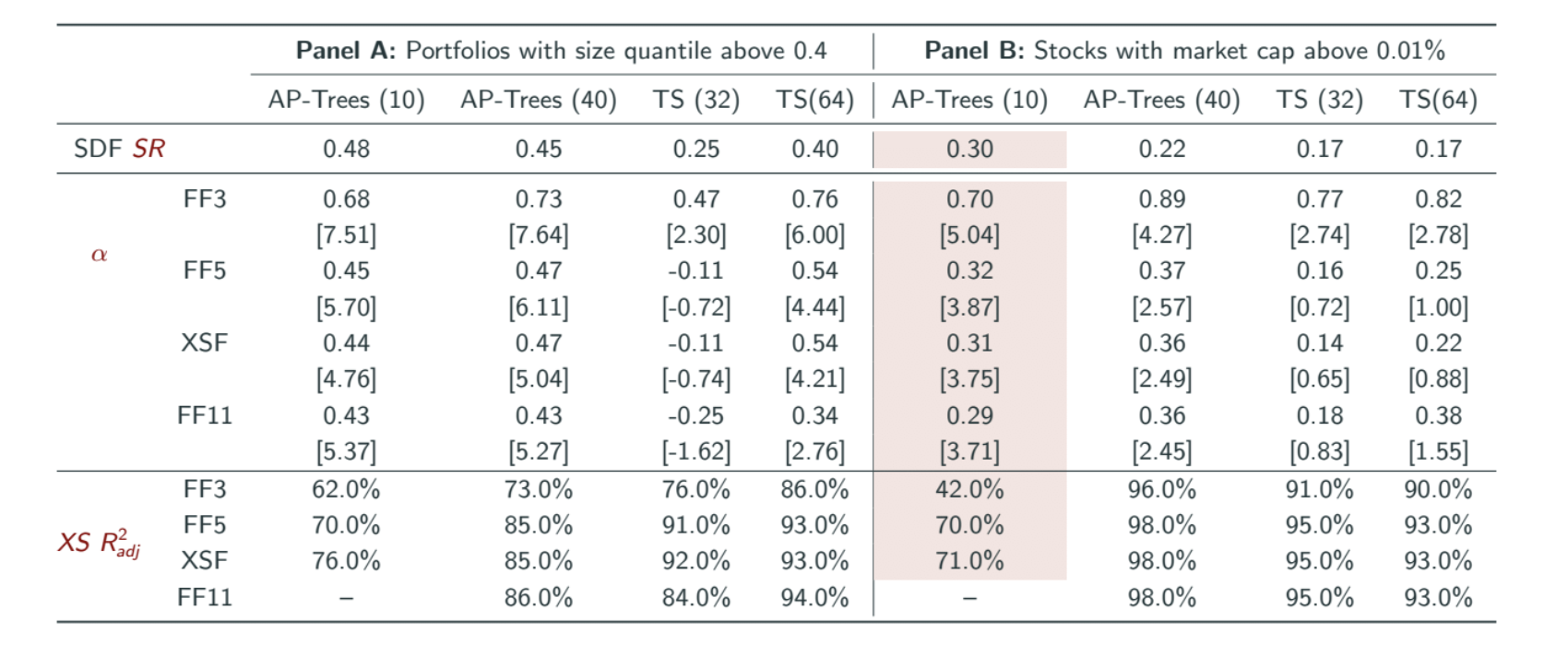
We could further check for turnover, rebalancing frequency, portfolio weights, time variation etc. and it is also a demonstration of how to include constraints like liquidity.
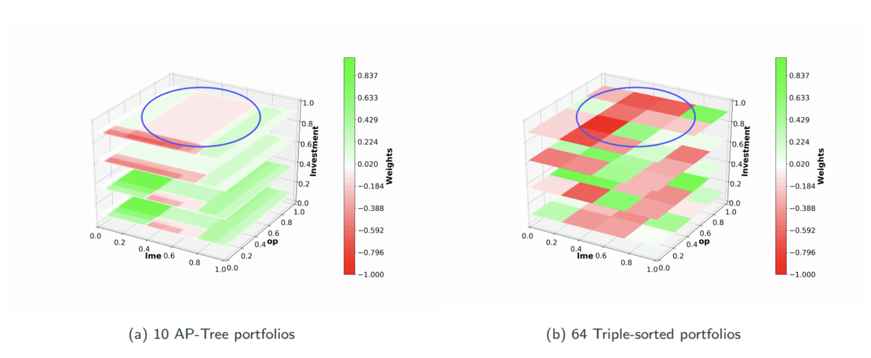
We also show the optimal portfolio loadings in the characteristics space, from the charts we know conditional interaction matters and triple sorting is just too coarse (the optimal combination loads on extremes on the spectrum)
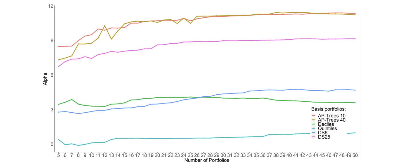
Now if we combine all 10 characteristics and form the testing portfolios using trees, deciles, and double-sorting. We see that AP-Trees double the Sharpe Ratio of stacked decile sorted portfolios. A small number of basis assets (20-30) for Tree-based portfolios is good enough to capture pricing signals. Moreover AP-Tree extract new pricing signal since the optimal portfolios (SDF) are not priced by the 11 risk factor models.
Conclusion
As a quantitative research in a hedge fund, our fundamental problems could be roughly categorized into two types
- Prediction signal (simple prediction): which is to find signal that predict future security returns. We could use
- Linear regression (most commonly used)
- Nonparametric prediction (e.g. kernel regression)
- Machine learning (e.g deep neural network or tree based approaches) to find such signals.
- Portfolio construction (ultimate goal of interest): we need to devise a portfolio to trade based on the prediction output. We could construct the portfolio using
- Long-short hedged strategies (highest decile minus lowest decile, risk factor mimicking)
- Mean-variance optimization Meanwhile we are facing portfolio constraints related to rebalancing, trading frictions, transaction costs, etc.
However the best overall prediction signals are NOT necessarily the best input for portfolio construction. So far machine learning techniques often focus unconditionally on step 1 when it comes to the finance realm. This paper is about extracting signal that is optimal for portfolio construction. It levers a joint approach to prediction signal and portfolio construction based on stock characteristics. It retains most benefits of traditional “machine learning” and is easily interpretable.
Why is machine learning useful for investment? Generically speaking:
- It is good at extracting signals from a large information set;
- It could easily capture complex nonlinear/interactive relationships among variables;
- It works well out-of-sample and is robust to overfitting.
On the other end, the natural pitfalls of machine learning includes:
- ML-based portfolios might be exposed to micro-caps stocks, which incur large turnover and transaction costs.
- ML-based portfolio construction is like a niche “black-box” approach and is not easy to sell to an average client.
- Asset returns in efficient markets are dominated by unforeseeable news, it is very hard to extract predictors out of data with such low signal to noise ratio.
This paper showcases how to combine economic structure with machine learning by building cross-sections of portfolios (SDF) using decision trees designed directly for investment strategies. This SDF is simple and interpretable, can adapt the selection of the assets and the depth of sorting. It is not driven by micro-caps and can easily extended to incorporate restrictions, transaction costs, etc., and it have not been over-studied yet.