Athans Blog

GRU, LSTM, and RNN application architectures

Gated RNNs

GRU

Gates are used in GRU and LSTM, these are not digital gates here. They generate gate signals $\Gamma$ ranging from 0 to 1. Usually $\Gamma$ is produced by sigmoid function $\sigma(x)$ whose output ranges from 0 to 1. It is used to mix two signals a and b as convex combination: $\Gamma a+(1-\Gamma)b$ or scale a signal (considering b to be 0) $\Gamma a$.

In order to introduce GRU, we first redraw the Jordan RNN where $\tilde s_i=tanh(w_c[x_i, s_{i-1}]), y_i=s_i=g_2(w_{sy}\tilde s_i)$ like below:

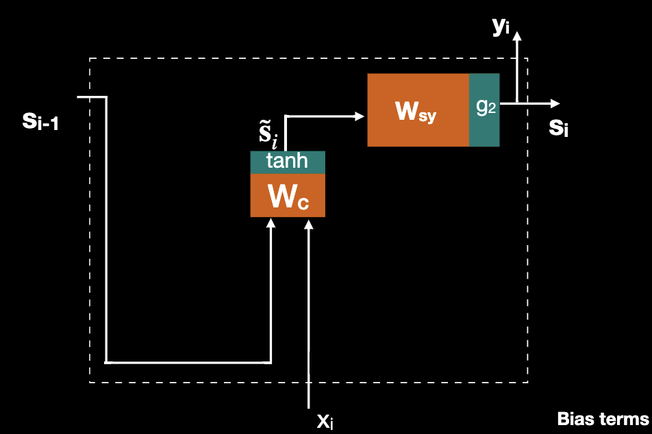
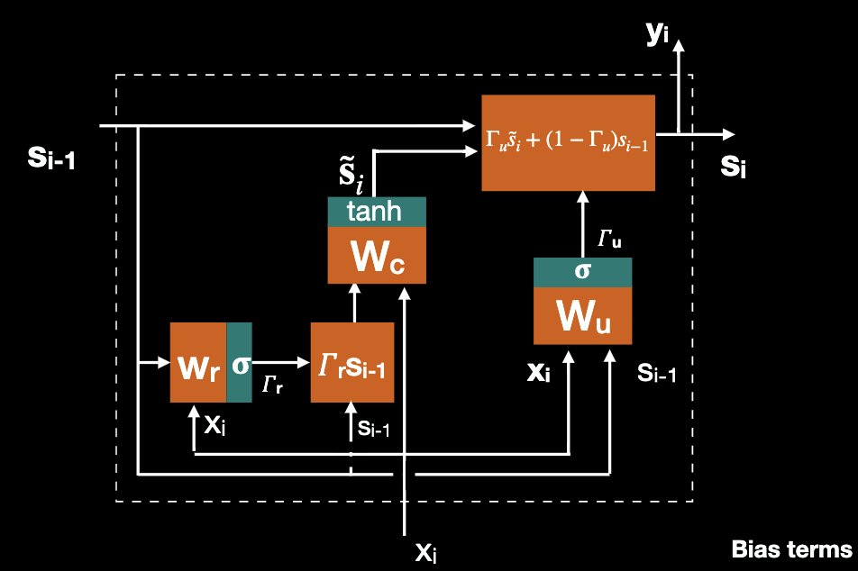
If we add an update gate $\Gamma_u$ in parallel to the hidden state, then we have a simple GRU where Where $\Gamma_u=\sigma(w_u[s_{i-1},x_i]+b_u), \tilde s_i=tanh(w_c[x_i, s_{i-1}]+b_c), y_i=s_i=\Gamma_u\tilde s_i+(1-\Gamma_u)s_{i-1}$

Further adding a reset gate $\Gamma_r$ and we formulate the full GRU, where $\Gamma_u=\sigma(w_u[s_{i-1},x_i]+b_u), \Gamma_r=\sigma(w_r[s_{i-1},x_i]+b_r)$ $\tilde s_i=tanh(w_c[x_i, \Gamma_r s_{i-1}]+b_c), y_i=s_i=\Gamma_u\tilde s_i+(1-\Gamma_u)s_{i-1}$

LSTM networks

LSTM stands for long short term memory, and the network has feedback for both state and output. LSTM differs from GRU where there are three gates for LSTM and two for GRU; More subtly, LSTM has 2 “state channels”, 4 layers with four weight matrices: $W_f, W_c, W_i, W_o$, and 3 gates.

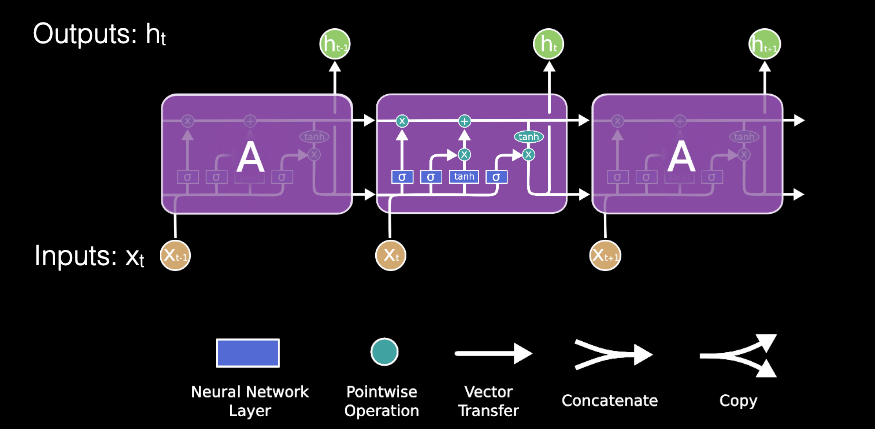
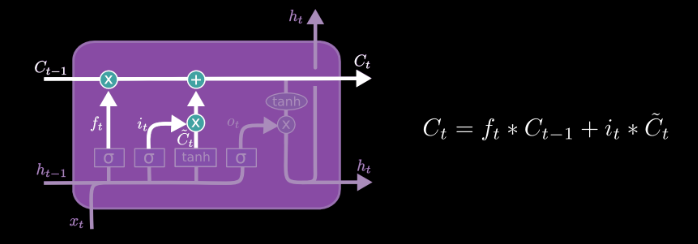
Now let’s look at the different components that make up an LSTM. The two state channels $h_t$ which the output $h_t$ is also fed back to the LSTM unit, $C_t$ which represents additional state information. The cell state $C_t$ is carried forward from one time instance to the next, $C_t$ is modified along the way. Note that state isa vector not a scalar.

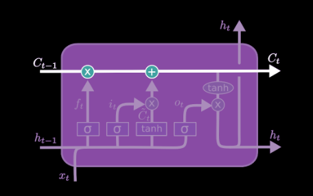
An LSTM “gate” makes an element wise decision on what to allow through. It is a fully connected layer followed by a sigmoid with outputs between 0 and 1. It’s like one of the gates in a GRU.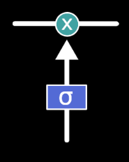

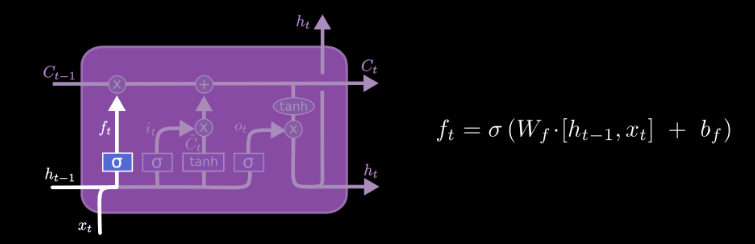
The forget fate decides what elements of the previous cell sate should be forgotten. When an element of $f_t$ is zero, the output of date is zero (forgotten).

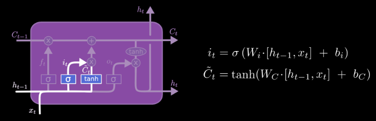
The input gate $i_t$ determines what new information from $\tilde C_t$ should be added to create the new cell state, where $\tilde C_t$ is the output of full connected layer gives proposed next state change. This new information is linearly transformed and then squashed by the tanh function which forces the output to lie between -1 and 1.

Outputs from the forget gate and the input gate combine to update the current cell state. Note that GRU took convex combination of C and $\tilde C$.

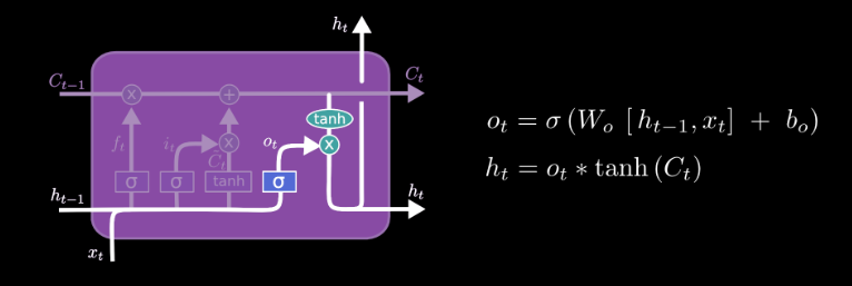
The output gate decides what information from the cell state should be output by the LSTM.

In general, LSTM has 3 gates, more parameters and have been more proven, while GRU has 2 gates, fewer parameters and is better trained on small datasets. Both are implemented in major frameworks and easy to use.

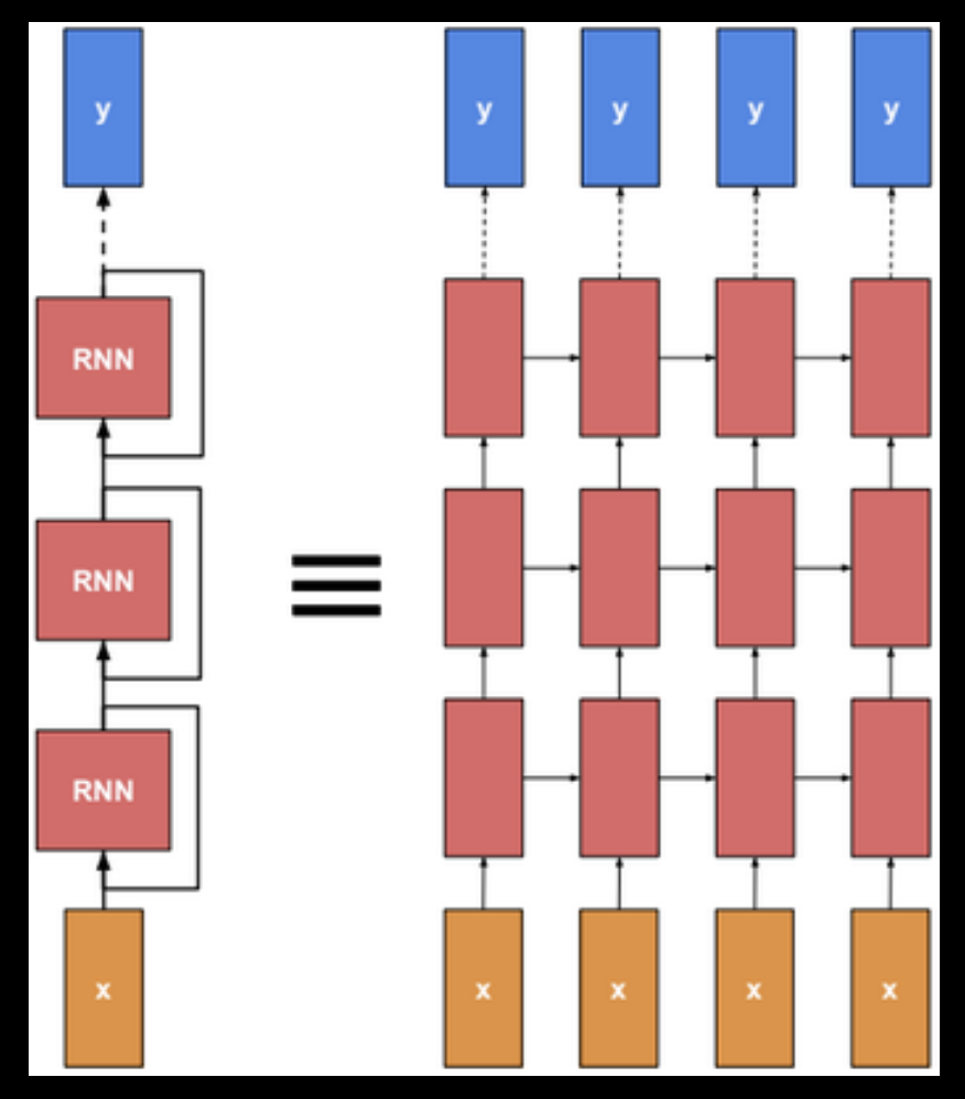
Bidirectional RNN, Multilayer RNN

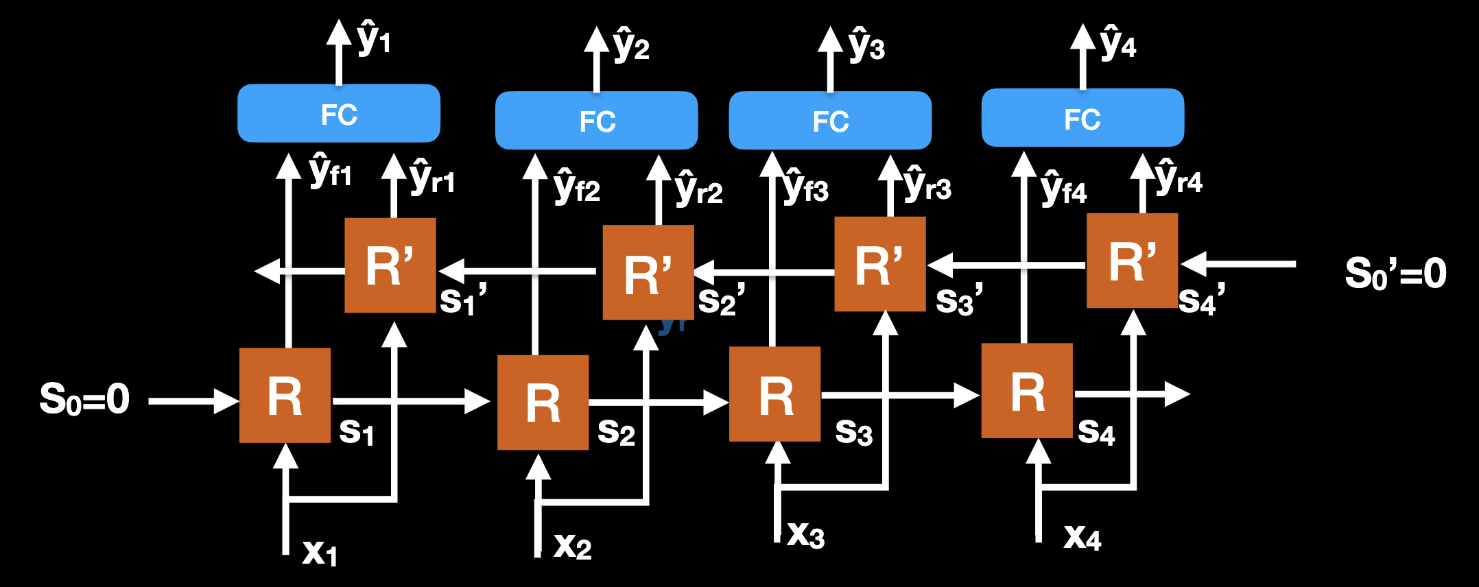
Bidirectional RNN are formed by two independent RNNs (can be any type), in which the forward direction is as usual, the reverse direction starts at end of the sequence and goes backward to start. Once forward and reverse RNNs are complete, outputs for each time step are concatenated, and may be passed through fully connected layer.

Multilayer RNN can be any RNN type like LSTM or GRU, it can be directional, it can have any number of layers (usually 2 or 3 layers). Sometimes it is called “Deep RNN”, its backdrop depth is really governed by unrolled sequence length, although number of parameters by layers.

RNN Application Architectures

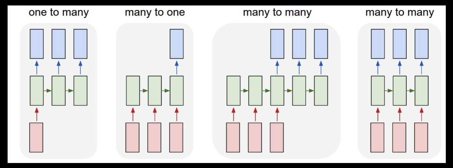
• One to Many

  The one to many architecture applies to sequence generation like audio or speech generation, or image caption generation. Its loss function is defined over all outputs.

• Many to One

  The Many to one architecture applies to sequence classification like sentiment analysis, video classification or stock market “Buy/Sell” decision. Its loss function is defined over single output and is usually cross entropy.

• Many to Many (same length)

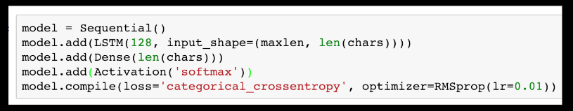
  It is usually used for classifying elements of a sequence such as Named Entity classification, video segmentation/activity labeling, statistical language model (char RNN), and some approaches to speech recognition. Its loss function is defined over all outputs and is usually sum of losses for each output.

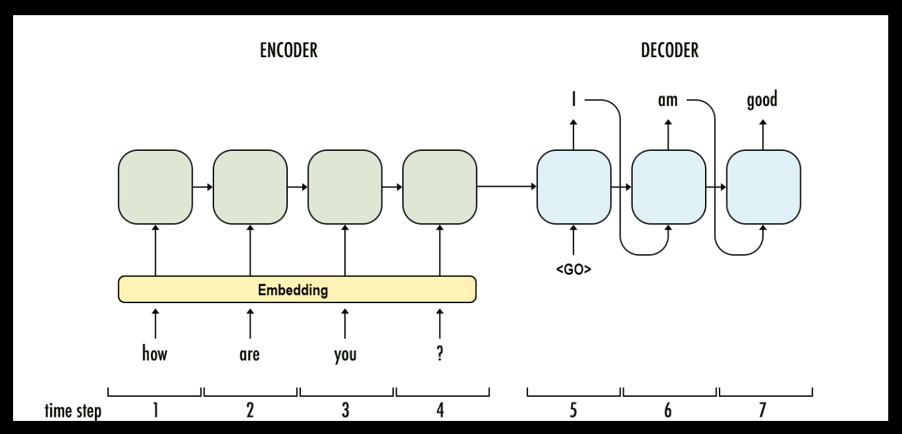
• Many to Many (different length)

  This architecture is often called Encoder-Decoder architecture with two RNNs. The input sequence is encoded into a vector, the output sequence is generated from such vector. It is widely used in language translation, video captioning, and Question-Answering.

  

Inference with beam search

In sequence generation or sequence-to-sequence problems, we want to find $\hat Y = argmax_{y_i \in Dict}\ P([y_1, y_2,...,y_T]|x)$ where x is the input (an image, a sequence etc.), and $[y_1, y_2,...,y_T]$ are over possible sequences where elements are from the Dictionary. In sequence to sequence architectures x is often the state s output by the encoder. Finding the maximum $P([y_1, y_2,...,y_T]|x)$ requires enumerating all sequences, which is exponential in sequence length.

We proposed earlier an inference method: $\hat y_1 = argmax\ P(y_1|x)$ ,$\hat y_2 = argmax\ P(y_2|\hat y_1,x)P(\hat y_1|x)$ , …, $\hat y_i = argmax\ P(y_i|\hat y_1,...,\hat y_{i-1}, x)P(\hat y_{i-1}|\hat y_1,...,\hat y_{i-2},x)...$

This is NOT optimal, it’s a greedy “best first” search.

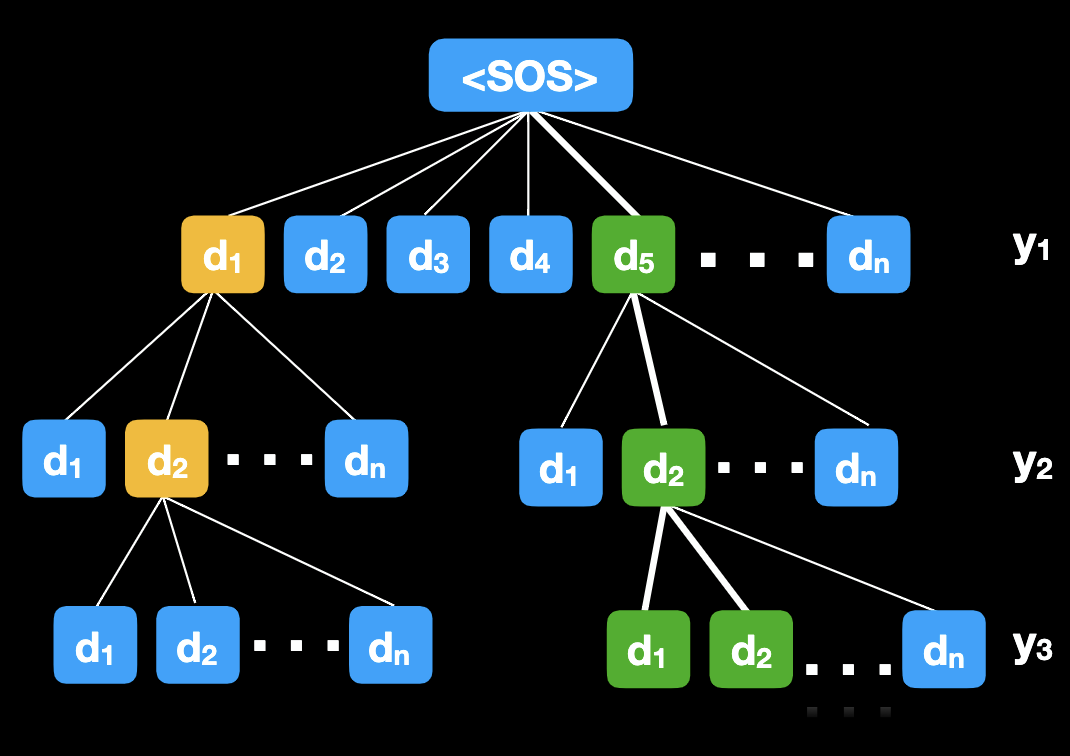
Inference can be viewed as searching a tree where the number of children of each node is the size of the Dictionary. Inference is a path through such tree. Exhaustive search is prohibitive due to the exponential complexity. Beam Search with beam size $\beta$, goes layer by layer and explores $\beta $ paths through the tree with highest probability. Search ends when <EOS> is selected or max length is reached. This term is introduced for speech recognition by Raj Reddy in 1977.

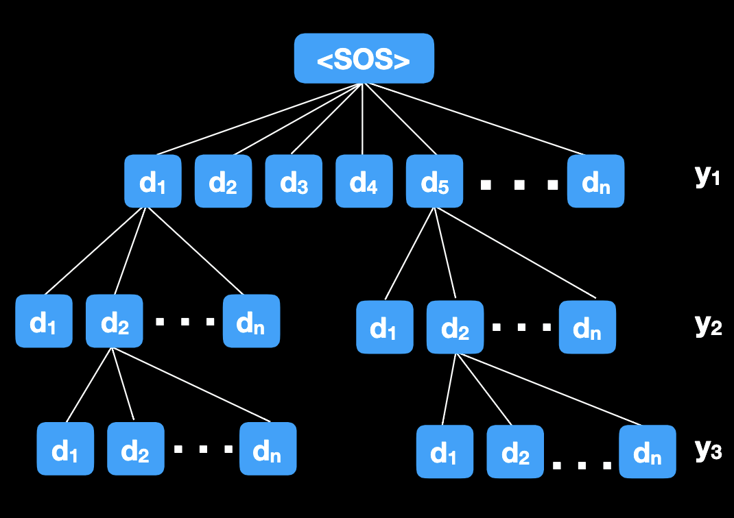
Let’s take Beam Search with $\beta =2$ as an example. We evaluate $p(d_i|x)$ for all $d_i$, retain two $d_i$ with largest $p(d_i|x)$ . Then we evaluate $p(d_i|x, \hat y_1)p(\hat y_1|x)$ for each $\hat y_1$ selected above and for all $d_i$, retain 2 paths $[\hat y_1, \hat y_2]$ with largest value. Similarly, we evaluate $p(d_i|x, \hat y_1, \hat y_2)p(\hat y_2|\hat y_1, x)p(\hat y_1|x)$ for each $\hat y_1, \hat y_2$ selected above and for all $d_i$, retain 2 paths $[\hat y_1, \hat y_2, \hat y_3]$ with largest value. We continue to deeper levels until <EOS> or max length etc.