Athans Blog

Sequence processing tasks with deep learning

Sequences

Sequence is an ordered list of elements, it could be infinite or finite, with fixed or variable length. The examples of sequence are discrete samples of an electric signal; characters in poem, Bid/Ask prices etc. The characteristics of the sequences are:

• Samples of “continuous” value like temperature, stock prices, audio etc. Sampled uniformly in time (or not)
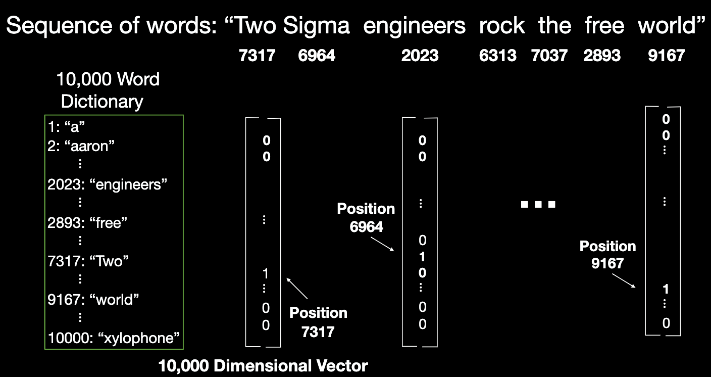
• Discrete values from a small set of possibilities (e.g. Roman characters, 1-10’s); Discrete values from a very large set of possibilities(e.g. words)
• High dimensional data (e.g. images)

Sequences are typically processed by digital signal processing model, finite state machines, learning automata, Markov models/Hidden Markov models, and our focus today: neural networks.

To give the notations for input/output sequences:

• Input sequence of length $T_x$: $x=(x_1, x_2, ..., x_{T_x})$
• Output sequence of length $T_y$: $y=(y_1, y_2, ..., y_{T_y})$

Input and output sequence elements may be in different types (e.g. text to speech). Input length could be 0,1, or arbitrary length $T_x$, output length could be 1, or arbitrary length $T_y$. Input length and output length could differ.

Examples of Sequence Modeling are list below:

We found direct application of the three sequence models highlighted above in the finance realm.

1. Sentiment classification. it’s just like extract sentiment from movie reviews.
2. Named entity recognition. it takes a sequence of text as input, it gives it label for each word ( person, place, not a named entity) as output.
3. Prediction. When elements of sequence are real numbers, methods like linear extrapolation are often used, when elements are categorical (e.g. text), learning is needed.

Sequences Processing

The sequence processing can be modeled in different forms:

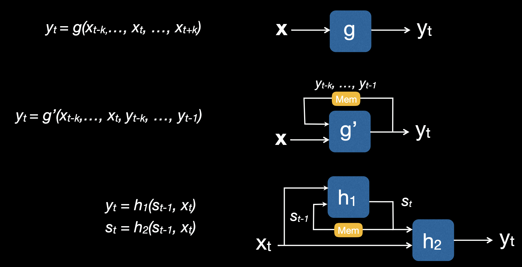
• General sequence processing: function f where $y=f(x)$
• Causal sequence processing with window size k+1: function g that is applied repeatedly for $t=1,...,T_y, y_t = g(x_{t-k}, x_{t-k+1},..., x_t)$
• Noncausal sequence processing with window size 2k+1: function g where $y_t = g(x_{t-k}, x_{t-k+1},..., x_t,...,x_{t+k})$
• Casual sequence processing being applied to both inputs and outputs: function g’ where $y_t = g(x_{t-k}, x_{t-k+1},..., x_t, y_{t-k}, y_{t-k+1},..., y_{t-1})$
• Recursive causal sequence processing, it introduce a new sequence state: $s_1,...,s_{T_x}$ and two update equations $h_1, h_2$, where $y_t=h_1(s_{t-1},x_t), s_t=h_2(s_{t-1},x_t)$

Put them graphically:

Causal sequence processing
$y_t = g(x_{t-k}, x_{t-k+1},..., x_t, y_{t-k}, y_{t-k+1},..., y_{t-1})$
can be re-written recursively where the state is simply k previous inputs and outputs
$s_{t-1}=[x_{t-k}, x_{t-k+1},..., x_{t-1}, y_{t-k}, y_{t-k+1},..., y_{t-1}]$
, and update is
$y_t=h_1(s_{t-1},x_t), s_t=h_2(s_{t-1},x_t)$
.For example, Exponential Moving Average (EMA) could be recursively written as
$y_t=\alpha x_t+(1-\alpha)y_{t-1}=\alpha x_t+(1-\alpha)[\alpha x_{t-1}+(1-\alpha)y_{t-2}]=\Sigma_i^\infin\alpha(1-\alpha)^ix_{t-i}$,
$where 0\leq \alpha \leq 1$ .

So the takeaways here are:

1. The state can include previous outputs.
2. Output of recursive processing can be affected by inputs from long ago (infinite past), and this is both good and bad, good because it provides long term memory well beyond the window size, bad because outlier inputs may have an effect that persists.

FeedForward Networks

Inference is the task that given x then we evaluate f(x). Classification is the kind of inference that given an input x, which of C classes is it?

Bayesian classifier defines $\hat C=argmax_{C_i} \ p(C_i|x)=argmax_{C_i} \ p(x|C_i)p(C_i)$ where $p(C_i|x)$ is the conditional probability of the class $C_i$ given the feature $x$. Bayesian classification is the best classifier ever…sort of. It’s the best because it has the lowest probability of error of any classier! And the “…sort of” lies in how should $p(C_i|x)$ be represented? How many training samples are needed? How do we learn $p(C_i|x)$ given a training set? How do we perform inference?

Nowadays we use multilayered network to train the model for inference. A single node of such network (or we say single layer network) looks like below:

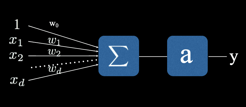
It’s modeled as: $y(x,w)=a(w^Tx+w_0)=a(w^Tx)$

Where x is the input vector padded with 1, w is the weights including bias, a is the activation function.

Activation function

We hereby list out the common types of activation functions:

• Sigmoid

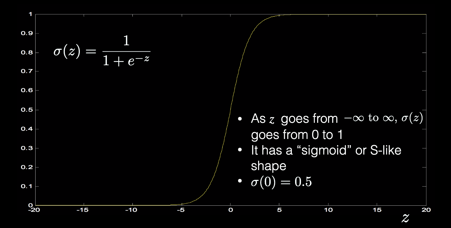
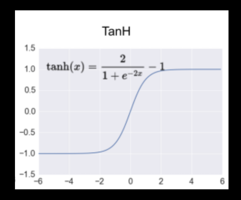
• Tanh

  As x goes from negative infinity to positive infinity, tank(x) goes from -1 to 1. It has a “sigmoid” or S-like shape, and tanh(0) = 0

  

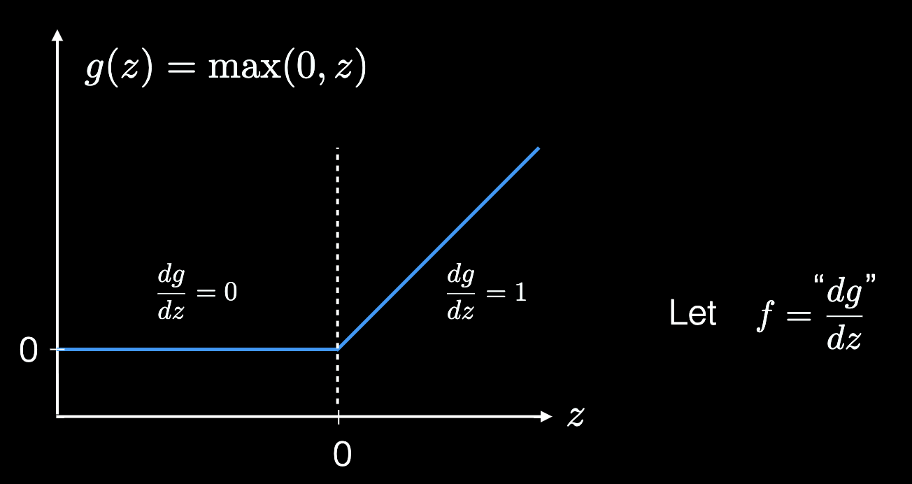
• Rectified Linear Unit (ReLU)

  

In the similar manner, a two layer network looks like below

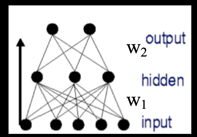
$y(x,w)=a_2(w_2^Ta_1(w_1^Tx+w_0))$, here we have two sets of weights, and weights for each layer are represented as a matrix; we also have two activation functions.

Feedforward Networks are composed of functions represented as “layers” $y(x)=a_3(a_2(a_1(x, w_1),w_2),w_3)$with weights $w_i$ associated with layer I and $a_i$ is the activation function for layer i. Meanwhile $y(x)$ can be a scalar or a vector function.

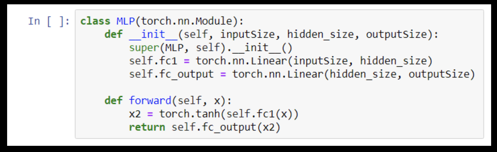
In PyTorch it is pretty simply to specify a two layer network.

To classify the input x into one of the C classes, we have C outputs $[y_1,...,y_c]$. Ideally, output $y_i$ is the posterior probability of class i given the input x. e.g. $y_i \approx p(C_i|x)$ . The outputs are positive, less than 1, and sum to 1: $\Sigma_{i=1}^Cy_i=\Sigma_{i=1}^Cp(C_i|x)=1$. Classification decision is $\hat C=argmax_i \ y_i\approx argmax_i \ p(C_i|x)$ . If the network were certain about the class, one output would be 1 and rest would be zero. This can be implemented with a softmax layer where z is the output of the previous layer $y_i(z) = \frac{e^{Z_i}}{\Sigma_{j=1}^Ce^{Z_j}}$.

Universal Approximation Theorem

If we have enough hidden units (one or more hidden layers) we can approximate “any” function with a two layer network.

So even though “any” function can be approximated with a. Network with single hidden layer, the network may fail to train, overfit, fail to generalize, or require so many hidden units as to be infeasible. This is both encouraging and discouraging.

However, academia showed that deeper networks are more efficient in that a deep rectified net can represent functions that would require an exponential number of hidden units in a shallow one hidden layer network. Deep networks composed on many rectified hidden layers are good at approximating functions that can be composed from simpler functions. And lots of taks such as image classification may fit nicely into this space.

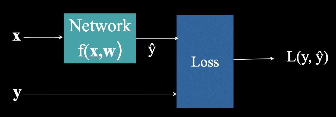
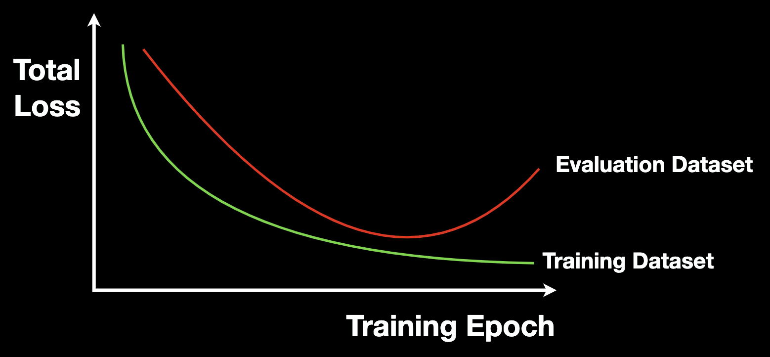
Training data is a set of sequences pairs $\{ <x^i, y^i>, 1\leq i\leq n\}$. Total Loss is a function $TL(w)=\Sigma_{i=1}^nL(f(x^i,w),y^i)$. Training is to find a w that minimize the total loss.

Loss function

Among the aforementioned, the loss function is really important. It's how we compare the network output to the training labels. We list out the common loss functions below

• Regression problems:
  • Distance: $L(y, \hat y) = ||y-\hat y||^p$, usually p=1 or 2
• Classification problems
  • Cross Entropy: $L(y, \hat y) =\Sigma_{i=1}^ny_ilog\frac{1}{\hat y_i}=-\Sigma_{i=1}^ny_ilog\hat y_i$ , where y is a vector with one 1 and rest 0s,$\hat y$ is a vector with positive floats that sum to 1 (output of Softmax).

Cross entropy between the output of a network $\hat y$ and ground truth y is commonly used when n classes are mutually exclusive. That is $\Sigma_{i=1}^ny_i=1$ . since y is “one hot”, only one term of the sum is non-zero, and there is only a positive loss back propagating from that one output.

Cross entropy is the number of bits we’ll need if we encode symbols from y using the wrong distribution of $\hat y$ . Minimizing cross entropy is minimizing the number of bits. It’s the same as minimizing the KL divergence between y and $\hat y$ . Maximizing the likelihood of the output $P(y|\hat y)=\Pi_{i=1}^nP(y_i|\hat y_i)$ is the same as minimizing the cross entropy.

Given a training set $\{ <x^i, y^i>, 1\leq i\leq n\}$ , estimate (learn) w by making $TL(w)=\Sigma_{i=1}^nL(f(x^i,w),y^i)$ small. In this training procedure we need:

• Back propagation using Stochastic Gradient Descent
• Adagrad, RMSprop, ADAM
• Regularization: Dropout, Batch/Group/Instance Normalization
• Early Stopping

Feedforward Network for processing sequences

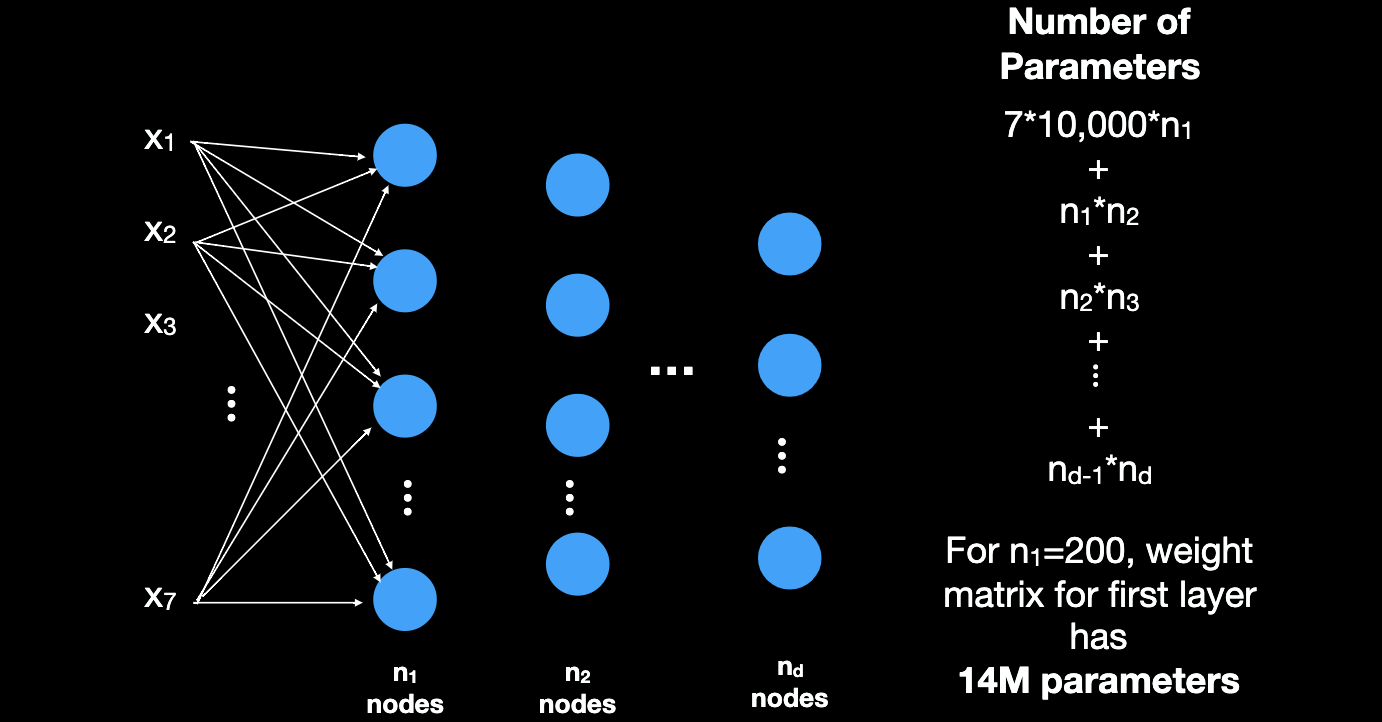
However there are problems with Feedforward Network for NLP:

1. Number of network weights become explosive in sequence length.

   

2. Input size is fixed.

3. Padding is possible, but then maximum sequence length means network is big. (First layer: Dictionary size * largest sequence length).

   

4. Output length is also fixed.

5. Doesn't share feature (weights) across sequence positions (harder to learn shift invariants).